4.3.10. Elevate operator

The Elevate operator uses a scalar field on a 2D mesh to elevate each node in the input mesh, resulting in a topologically 2D surface in 3D. The Elevate operator allows you to perform much of the same functionality as a Surface plot and it allows you to do additional things like elevate plots that do not accept scalar variables. The Elevate operator can also elevate plots whose input data was produced from higher dimensional data that has been sliced. Furthermore, the Elevate operator allows you to display multiple scalar fields in a single plot such as when a Pseudocolor plot of scalar variable A is elevated by scalar variable B (see: Figure 4.32).

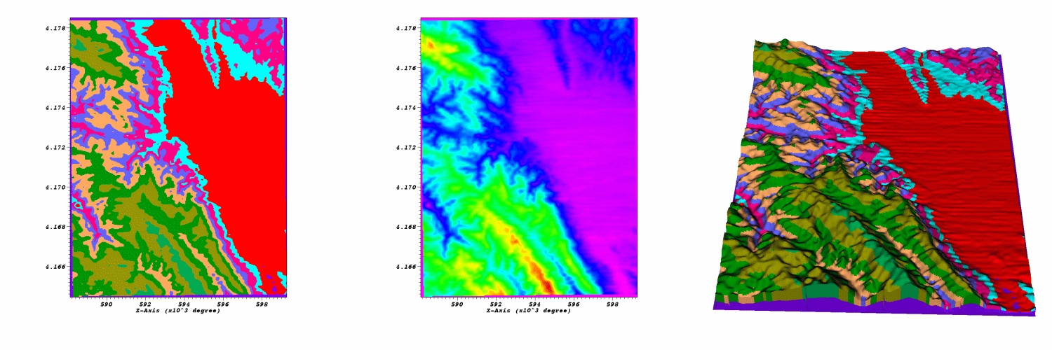
Fig. 4.32 Elevate operator example: 2D plot of rainfall; 2D plot of elevation; Plot of rainfall elevated by elevation

4.3.10.1. Using the Elevate operator

The Elevate operator can be used to create plots that look much like a Surface plot if you simply apply the Elevate operator to a plot that accepts scalar values. The Elevate operator is more flexible than a Surface plot because whereas the Surface plot limits you to elevating by one variable and coloring by the same variable, the Elevate operator can be used with any plot and still achieve the Surface plot’s elevated effect. You could use the Elevate operator to elevate a Pseudocolor plot of rainfall by elevation. You could also take Vector or FilledBoundary plots (among others) and elevate them by a scalar variable.

Since the Elevate operator uses a scalar variable to elevate all of the points in the mesh, the Elevate operator has a number of controls related to scaling scalar data. For example, the Elevate operator allows you to artificially set minimum and maximum values for the scalar variable so you can eliminate data that might otherwise cause your elevated plot to be stretched undesirably in the Z direction. To set minimum and maximum values for the Elevate operator, click on the Min or Max check boxes in the Elevate attributes window (see Figure 4.33) and type new values into the adjacent text fields. The options for scaling the plots created using the Elevate operator are the same as those for scaling Surface plots. For more information on scaling, see the Surface plot documentation.

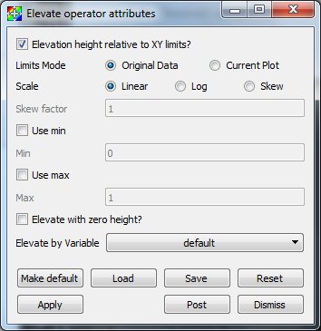
Fig. 4.33 Elevate window

The most useful feature of the Elevate operator is its ability to elevate plots using an arbitrary scalar variable. By default, the Elevate operator uses the plotted variable in order to elevate the plot’s mesh. This only works when the plotted variable is a scalar variable. When you apply the Elevate operator to plots that do not accept scalar variables, the Elevate operator will fail unless you choose a specific scalar variable using the Elevate by Variable variable menu in the Elevate attributes window.

4.3.10.2. Changing elevation height

The Elevate operator uses a scalar variable’s data values as the Z component when converting a mesh’s 2D coordinates into 3D coordinates. When the scalar variable’s data extents are small relative to the mesh’s X and Y extents then you often get what appears to be a flat 2D version of the data floating in 3D space. It is sometimes necessary to scale the scalar variable’s data extents relative to the spatial extents in order to produce a visualization where the Z value differs noticeably. If you want to exaggerate the Z values that the scalar variable contributes to make differences more obvious, you can click on the Elevation height relative to XY limits check box in the Elevate attributes window.

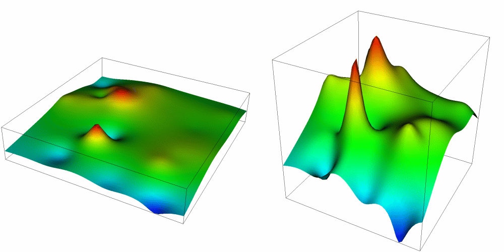
Fig. 4.34 Effect of scaling relative to XY limits

The Elevate operator can be used to simply place a 2D plot in 3D space by use of the Elevate with zero height option. This will assign a value of zero to all of the z coordinates when converting into 3D.

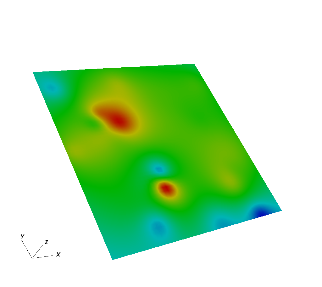
Fig. 4.35 Effect of elevating with zero height