4.3.14. Integral Curve System
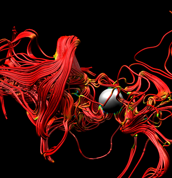
Within the VisIt infrastructure is the ability to generate integral curves. An integral curve is a curve that begins at a seed location and is tangent at every point in a vector field. It is computed by numerical integration of the seed location through the vector field. For example, the image below shows integral curves through the magnetic field of a core-collapse supernova simulation from the GenASiS code.
The generation of integral curves forms the basis of VisIt’s Integral Curve System (ICS), made up of the Integral Curve operator, the Lagrangian Coherent Structure (LCS) operator, the Limit Cycle operator, and the Poincaré operator. Much of the underlying infrastructure and interface is the same for each operator: the user selects a series of seed locations where curves are generated, which are then visualized and analyzed.
The ICS allows for the computation of Lagrangian Coherent Structures (LCS)
using a variety of techniques developed by George Haller and his group at ETH Zürich. For more information
on LCS, see K. Onu, F. Huhn, & G. Haller, LCS Tool: A Computational
platform for Lagrangian coherent structures, J. of Computational Science, 7
(2015) 26-36.
Many of the terms used in the ICS are familiar to experts in dynamical systems
but may be new to many users. Users can refer to a glossary sepcific to dynamical systems and can reference
VisIt’s Glossary for some terms that are specific to VisIt’s ICS. Any
additional terms can be defined through a simple online search.
4.3.14.5. Parameters
Common to all ICS operators is a four tab GUI: Source, Integration, Appearance, and Advanced (the Poincaré operator also has an Analysis tab). These tabs contain many functions that are common across all four operators. The following is a description of those common features.
4.3.14.5.1. Source
The set of points that seed the integral curves. See each operator for varied settings.
4.3.14.5.1.1. Field
Sets the field type so that the native elements are used when interpolating the vector fields. Each operator provides the following options:
Warning
Each option below besides “Default” requires the respective third party library.
- Default
Use VisIt’s native VTK mesh structure to perform linear interpolation on the vector field.
- Flash
Evaluates the velocity field via the Lorentz force. Parameters are:
Constant - A constant multiple applied to the velocity.
Velocity - When combined with Leap-Frog integration, this sets the initial velocity used in the integration.
- M3D-C1 2D
Evaluates the 3D magnetic field via a 2D poloidal 6th order polynomial. Parameters are:
Constant - A constant multiple applied to the perturbed part of the field.
- M3D-C1 3D
Evaluates the 3D magnetic field via a 2D poloidal 6th order polynomial and 1D toroidal 4th order Bezier spline.
- Nek5000
Evaluates the 3D vector field using Nek5000 spectral elements.
- Nektar++
Evaluates the 3D vector field using Nektar++ spectral elements.
4.3.14.5.2. Integration
Specify settings for the numerical integrator. See each operator for varied settings.
4.3.14.5.2.1. Integrator
Sets the integration scheme. There are various options common among numerical integration packages, such as Leap Frog and Runge-Kutta. More details on the different schemes can be found through a simple online search.
4.3.14.5.2.2. Step Length
Most integrators use a fixed step length. Runge-Kutta-Dormand-Prince (RKDP) uses adaptive step size, which can be clipped by the step length.
4.3.14.5.2.3. Tolerances
RKDP, Adams-Bashforth, and MD3-C1 make use of the tolerance options.
- RKDP
The step size adapts to ensure that the maximum error at each step is less than the maximum between the absolute tolerance and the relative tolerance times the value of the vector field at the current point. The absolute tolerance can be truly absolute or relative to the bounding box.
4.3.14.5.2.4. Termination
The criteria for terminating the integration. See specific operator for details.
4.3.14.5.3. Appearance
Specify appearance settings for the curves. See each operator for varied settings.
4.3.14.5.3.1. Streamlines vs Pathlines
The user may select the integral curve to be based on an instantaneous or time-varying vector field producing streamlines or pathlines, respectively. A streamline is a path rendered by an integrator that uses the same vector field for the entire integration. A pathline uses the vector field that is in-step with the integrator, so that as the integrator steps through time, it uses data from the vector field at each new time step. Pathline options are:
- Override starting time
Instead of starting with the current time step, utilize another time for the start time.
- Interpolation over time
Interpolate the integral curve with a static mesh for all time or with a varying mesh at each time step. The mesh is typically static, but this cannot always be assumed and should be verified for each dataset before use.
4.3.14.5.4. Advanced
4.3.14.5.4.1. Parallel integration
The user may select one of four different parallelization options when integrating curves in parallel:
- Parallelize over curves
Distribute the curves between the processors. Parameters are:
Domain cache size - number of blocks to hold in memory for level of details.
- Parallelize over domains
Distribute the domains between the processors. Parameters are:
Communication threshold - number of integral curve to process before communication occurs.
- Parallelize over curves and domains
Distribute both the curves and domains between the processors.
- Have VisIt select the best algorithm
VisIt automagically selects the best parallelization algorithm.
4.3.14.5.4.2. Warnings
Alerts for various conditions that may occur during the integration or analysis.
- Issue warning when the maximum number of steps is reached
The maximum number of steps limits run-a-way integration.
- Issue warning when a step size underflow is detected
If the step size goes to zero, issue a warning.
- Issue warning when stiffness is detected
Stiffness refers to one vector component being so much larger than another that tolerances can’t be met.
- Issue warning when a curve doesn’t terminate at a critical point
For example, the curve may circle around a critical point without converging.