5. The PlainText file format

Standard CSV (Comma Separated Values) files are read using the PlainText reader.

Plain text files are text files with columns of data. A single space, comma or tab character separates (e.g. delimits) values in each line of the file belonging to the different columns. The PlainText reader automatically detects the separator character in use. The file can include an arbitrary number of lines at the beginning of the file to be skipped. Following any skipped lines, the file may include an optional header line holding the names associated with each column. Plain text files can be used to represent the following types of data:

• A collection of curves, all defined on the same (explicit or implicit) domain.

• Points in 2D or 3D with variables defined on the points.

• A single variable defined on a 2D, uniform grid.

5.1. Defining curves with a PlainText file

The first line can be an optional list of variable names. The remaining lines consist of rows, where each row represents one point in each of the curves. In this example, the values on each row are separated by commas.

Here are the first 10 lines of an example of a file representing curves.

angle,sine,cosine
0,0,1
5,0.0871557,0.996195
10,0.173648,0.984808
15,0.258819,0.965926
20,0.34202,0.939693
25,0.422618,0.906308
30,0.5,0.866025
35,0.573576,0.819152
40,0.642788,0.766044

Here is the Python script that created the file.

    with open(filename, "wt") as f:
        # create header
        f.write("angle,sine,cosine\n")
        npts = 73
        for i in range(npts):
            angle_deg = float(i) * (360. / float(npts-1))
            angle_rad = angle_deg * (3.1415926535 / 180.)
            sine = math.sin(angle_rad)
            cosine = math.cos(angle_rad)
            # write abscissa (x value) and ordinates (y-value(s))
            f.write("%g,%g,%g\n" % (angle_deg, sine, cosine))

Here are the PlainText reader options used to read the data.

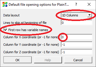
If you specify the column for the X coordinates, then that column will be used for the domain for all the curves. If you don’t specify an X coordinate, then it will use the row index for the domain for all the curves.

Here is the Python code to plot this data in VisIt

    plainTextOpenOptions = GetDefaultOpenOptions()
    plainTextOpenOptions['First row has variable names'] = 1
    plainTextOpenOptions['Column for X coordinate (or -1 for none)'] = 0
    SetDefaultFileOpenOptions("PlainText", plainTextOpenOptions)

    OpenDatabase("curves.csv")
    AddPlot("Curve","sine")
    AddPlot("Curve","cosine")
    DrawPlots()

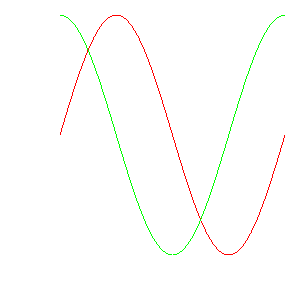
and the resulting data plotted in VisIt

5.2. Defining curves using row index for X coordinate

Here are the first 10 lines of an example of a file representing curves where the abscissa (e.g. x-coordinate) is implied by the row number (starting from 0) in the file. In this example, the values on each row are separated by commas.

inverse,sqrt,quadratic
100,0,0
50,10,0.01
33.3333,14.1421,0.04
25,17.3205,0.09
20,20,0.16
16.6667,22.3607,0.25
14.2857,24.4949,0.36
12.5,26.4575,0.49
11.1111,28.2843,0.64

Here is the Python script that created the file.

    with open(filename, "wt") as f:
        # create header
        f.write("inverse,sqrt,quadratic\n")
        npts = 100 
        for i in range(npts):
            inv = float(100) / (float(i)+1)
            sqr = 10 * math.sqrt(i)
            quad = float(i*i) / float(100)
            f.write("%g,%g,%g\n" % (inv, sqr, quad))

Here is the Python code to plot this data in VisIt

    plainTextOpenOptions = GetDefaultOpenOptions()
    plainTextOpenOptions['First row has variable names'] = 1
    SetDefaultFileOpenOptions("PlainText", plainTextOpenOptions)

    OpenDatabase("curves_nox.csv")
    AddPlot("Curve","inverse")
    AddPlot("Curve","sqrt")
    AddPlot("Curve","quadratic")
    DrawPlots()

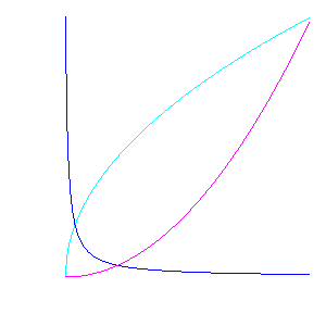
and the resulting data plotted in VisIt

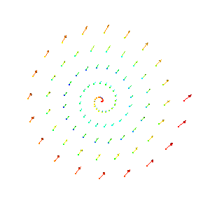
5.3. Defining 2D or 3D points with variables

The first line can be an optional list of variable names. The remaining lines consist of rows, where each row represents the coordinates and variable values for a single point. In this example, the values on each row are separated by spaces.

Here are the first 10 lines of an example of a file representing 3D points.

x y z velx vely velz temp
0 0 0 0 0 0 0.5
0.0959668 0.0315185 0.10101 0.10101 0.105813 0.139329 0.489899
0.162681 0.119779 0.20202 0.20202 0.23486 0.259379 0.479798
0.175775 0.246841 0.30303 0.30303 0.390843 0.35032 0.469697
0.119968 0.385819 0.40404 0.40404 0.558664 0.421475 0.459596
-0.00801311 0.504987 0.505051 0.505051 0.714204 0.505114 0.449495
-0.198223 0.572728 0.606061 0.606061 0.833862 0.637653 0.439394
-0.428209 0.56266 0.707071 0.707071 0.903623 0.826627 0.429293
-0.665597 0.45823 0.808081 0.808081 0.928962 1.04691 0.419192

Here is the Python script that created the file.

    with open(filename, "wt") as f:
        # write header
        f.write("x y z velx vely velz temp\n")
        n = 100
        for i in range(n):
            t = float(i) / float(n-1)
            angle = t * (math.pi * 2.) * 5.
            r = t * 10.
            x = r * math.cos(angle)
            y = r * math.sin(angle)
            z = t * 10.
            vx = math.sqrt(x*x + y*y)
            vy = math.sqrt(y*y + z*z)
            vz = math.sqrt(x*x + z*z)
            temp = math.sqrt((t-0.5)*(t-0.5))
            # write point and value(s)
            f.write("%g %g %g %g %g %g %g\n" % (x,y,z,vx,vy,vz,temp))

Here are the PlainText reader options used to read the data.

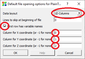
If you specify the columns for the X and Y coordinates, the points will be defined in 2D space. If you specify the columns for the X, Y and Z coordinates, the points will be defined in 3D space.

Here is the Python code to plot this data in VisIt

    plainTextOpenOptions = GetDefaultOpenOptions()
    plainTextOpenOptions['First row has variable names'] = 1
    plainTextOpenOptions['Column for X coordinate (or -1 for none)'] = 0
    plainTextOpenOptions['Column for Y coordinate (or -1 for none)'] = 1
    plainTextOpenOptions['Column for Z coordinate (or -1 for none)'] = 2
    SetDefaultFileOpenOptions("PlainText", plainTextOpenOptions)
    OpenDatabase("points.txt")

    DefineVectorExpression("vel", "{velx,vely,velz}")
    AddPlot("Pseudocolor", "temp")
    AddPlot("Vector","vel")
    DrawPlots()

and the resulting data plotted in VisIt

5.4. Defining a single variable on a 2D uniform grid

The data is interpreted as a node centered variable on a uniform mesh where the row and column indices define the X and Y coordinates. The rows represent values along the X direction and the rows get stacked in the Y direction. Each row further down in the file gets stacked up, one upon the other in the visualized result in VisIt. This means that the row-by-row downward direction in the file listing is the same as the upward (positive Y) direction in the visualized result in VisIt.

The first line can be an optional list of variable names. The first column name will be used for the name of the variable. Other column names are ignored but nonetheless required to read the file properly. The remaining lines consist of rows, where each row represents the values for a single Y coordinate.

Here is an example of a file listing representing 3D points. In this example, the values on each row are separated by spaces.

density c2 c3 c4 c5 c6 c7 c8
0 1 2 3 4 5 6 7
1 1.41421 2.23607 3.16228 4.12311 5.09902 6.08276 7.07107
2 2.23607 2.82843 3.60555 4.47214 5.38516 6.32456 7.28011
3 3.16228 3.60555 4.24264 5 5.83095 6.7082 7.61577
4 4.12311 4.47214 5 5.65685 6.40312 7.2111 8.06226
5 5.09902 5.38516 5.83095 6.40312 7.07107 7.81025 8.60233
6 6.08276 6.32456 6.7082 7.2111 7.81025 8.48528 9.21954
7 7.07107 7.28011 7.61577 8.06226 8.60233 9.21954 9.89949
8 8.06226 8.24621 8.544 8.94427 9.43398 10 10.6301
9 9.05539 9.21954 9.48683 9.84886 10.2956 10.8167 11.4018

Here is the Python script that created the file.

    with open(filename, "wt") as f:
        # Only the first column name matters.
        # The others are required but otherwise ignored.
        f.write("density c2 c3 c4 c5 c6 c7 c8\n")
        nx = 8
        ny = 10
        for iy in range(ny):
            y = float(iy)
            for ix in range(nx):
                x = float(ix)
                dist = math.sqrt(x*x + y*y)
                if (ix < nx - 1):
                   f.write("%g " % dist)
                else:
                   f.write("%g\n" % dist)

Here are the PlainText reader options used to read the data.

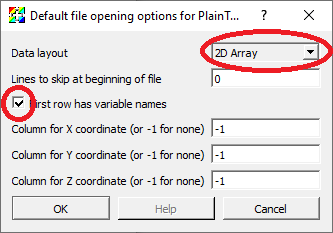
The columns for the X, Y and Z coordinates are not used.

Here is the Python code to plot this data in VisIt

    plainTextOpenOptions = GetDefaultOpenOptions()
    plainTextOpenOptions['First row has variable names'] = 1
    plainTextOpenOptions['Data layout'] = '2D Array'
    SetDefaultFileOpenOptions("PlainText", plainTextOpenOptions)

    OpenDatabase("array.txt")
    AddPlot("Pseudocolor", "density")
    DrawPlots()
    ResetView()

and the resulting data plotted in VisIt

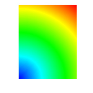
Note that the reddest part of the plot (e.g. highest numerical values in the data) appears in the upper right corner of the plot whereas the highest numerical values in the file data row-by-row listing appears in the lower right corner.