8.1. Expressions¶

Scientific simulations often keep track of several dozen variables as they run. However, only a small subset of those variables are usually written to a simulation database to save disk space. Sometimes variables can be derived from other variables using an expression. VisIt provides expressions to allow scientists to create derived variables using variables that are stored in the database. Expressions are extremely powerful because they allow users to analyze new data without necessarily having to rerun a simulation. Variables created using expressions behave just like variables stored in a database; they appear in menus where database variables appear and can be visualized like any other database variable.

8.1.1. Expression Window¶

VisIt provides an Expression Window, shown in Figure 8.1, that allows users to create new variables that can be used in visualizations. Users can open the Expression Window by clicking on the Expressions option in the Main Window’s Controls menu. The Expression Window is divided vertically into two main areas with the Expression list on the left and the Definition area on the right. The Expression list contains the list of expressions. The Definition area displays the definition of the expression that is highlighted in the Expression list and provides controls to edit the expression definition.

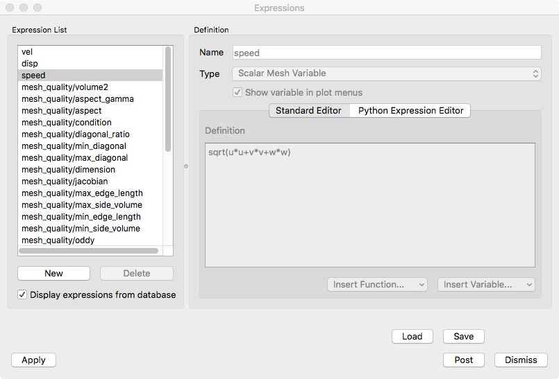
Fig. 8.1 Expression Window

Expressions in VisIt are created either manually by the user or automatically by various means including…

Preferences
- Mesh quality expressions
- Time derivative expressions
- Vector magnitude expressions
GUI wizards
Operators
Databases

By default, the Expression list will display only those expressions created manually by the user. A check box near the bottom of the Expression list controls the display of automatically created expressions. When this box is checked, the Expression list will also include expressions created automatically by Preferences and Databases but not expressions created automatically by GUI wizards or Operators.

8.1.1.1. Creating a new expression¶

Users can create a new expression by clicking on the Expression Window’s New button. When the user clicks on the New button, VisIt adds a new expression and shows its new, empty definition in the Definitions area. The initial name for a new expression is “unnamed” followed by some integer suffix. After the user types a new name for the expression into the Name text field, the expression’s name in the Expression list will update. If the user types a name that already exists in the expression list, then Visit will automatically append a number to the end of the name to avoid duplicate expression names.

Each expression also has a Type that specifies the type of variable the expression produces. The available types are:

Scalar
Vector
Tensor
Symmetric Tensor
Array
Curve

Users must be sure to select the appropriate type for any expression they create. The selected type determines the menu in which the variable appears and subsequently the plots that can operate on the variable.

To edit an expression’s definition, users can type a new expression comprised of constants, variable names, and even other VisIt expressions into the Definition text field. The expression definition can span multiple lines as the VisIt expression parser ignores whitespace. For a complete list of VisIt’s built-in expressions, refer to the table in section Built-in expressions. Users can also use the Insert Function… menu, shown in Figure 8.2, to insert any of VisIt’s built-in expressions directly into the expression definition. The list of built-in expressions is divided into certain categories as shown by the structure of the Insert Function… menu.

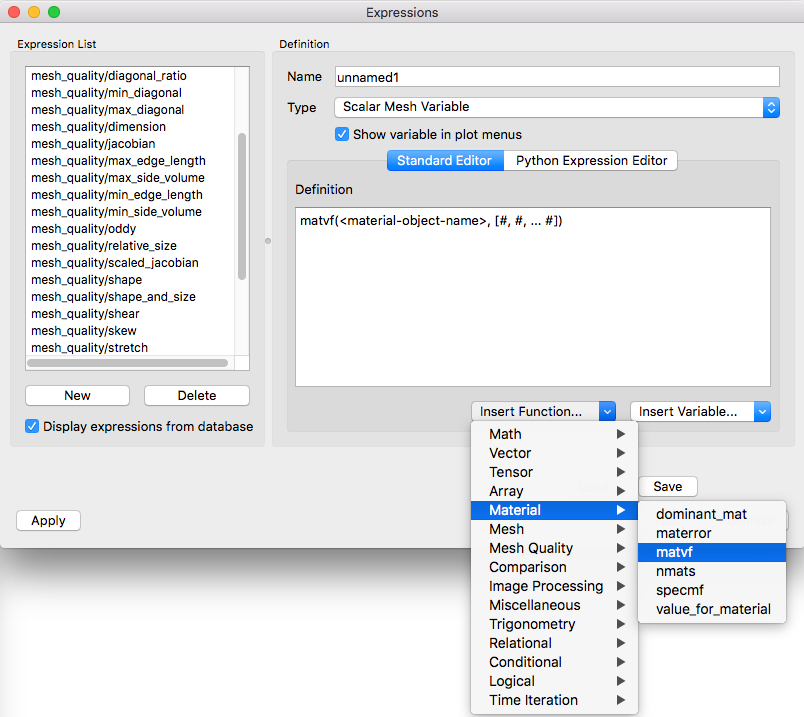
../../_images/expressionwindow-functionmenu.png

Fig. 8.2 Expression Window’s Insert Function… menu

In the example shown in Figure 8.2, the Insert Function… operation inserted a sort of template for the function giving some indication of the argument(s) to the function and their meanings. Users can then simply edit those parts of the function template that need to be specified.

In addition to the Insert Function… menu, which lets users insert built-in functions into the expression definition, VisIt’s Expression Window provides an Insert Variable… menu that allows users to insert variables from the active database into the expression definition. The Insert Variable… menu, shown in Figure 8.3, is broken up into Scalars, Vectors, Meshes, etc. and has the available variables under the appropriate heading so they are easy to find.

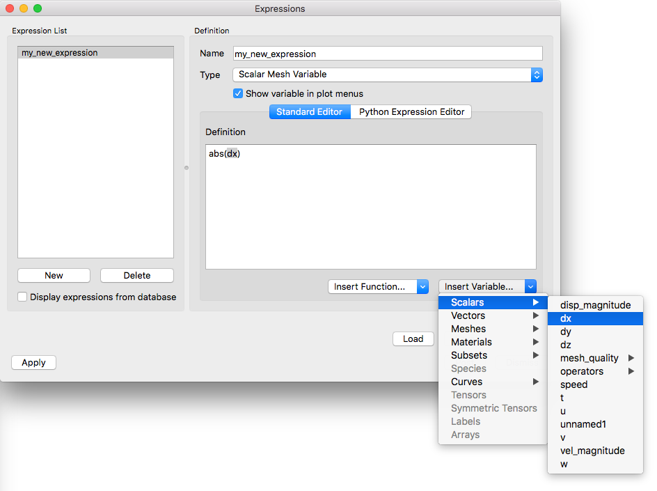
../../_images/expressionwindow-varmenu.png

Fig. 8.3 Expression Window’s Insert Variable… menu

Some variables can only be expressed as very complex expressions containing several intermediate subexpressions that are only used to simplify the overall expression definition. These types of subexpressions are seldom visualized on their own. If users want to prevent them from being added to the Plot menu, turn off the Show variable in plot menus check box.

8.1.1.2. Deleting an expression¶

Users can delete an expression by clicking on it in the Expression list and then clicking on the Delete button. Deleting an expression removes it from the list of defined expressions and will cause unresolved references for any other expressions that use the deleted expression. If a plot uses an expression with unresolved references, VisIt will not be able to generate it until the user resolves the reference.

8.1.2. Expression grammar¶

VisIt allows expressions to be written using a host of unary and binary math operators as well as built-in and user-defined functions. VisIt’s expressions follow C-language syntax, although there are a few differences. The following paragraphs detail the syntax of VisIt expressions.

8.1.2.1. Math operators¶

These include use of +, -, *, /, ^ as addition, subtraction, multiplication, division, and exponentiation as infix operators, as well as the unary minus, in their normal precedence and associativity. Parentheses may be used as well to force a desired associativity.

Examples: a+b^-c (a+b)*c

8.1.2.2. Constants¶

Scalar constants include floating point numbers and integers, as well as booleans (true, false, on, off) and strings.

Examples: 3e4 10 “mauve” true false

8.1.2.3. Vectors¶

Expressions can be grouped into two or three dimensional vector variables using curly braces.

Examples: {xc, yc} {0,0,1}

8.1.2.4. Lists¶

Lists are used to specify multiple items or ranges, using colons to create ranges of integers, possibly with strides, or using comma-separated lists of integers, integer ranges, floating points numbers, or strings.

Examples: [1,3,2] [1:2, 10:20:5, 22] [silver, gold] [1.1, 2.5, 3.9] [level1, level2]

8.1.2.5. Identifiers¶

Identifiers include function names, defined variable and function names, and file variable names. They may include alphabetic characters, numeric characters, and underscores in any order. Identifiers should have at least one non-numeric character so that they are not confused with integers, and they should not look identical to floating point numbers such as 1e6.

Examples: density x y z 3d_mesh

8.1.2.6. Functions¶

These are used for built in functions, but they may also be used for functions/macros defined by the user. They take specific types and numbers of arguments within the parentheses, separated by commas. Some functions may accept named arguments in the form identifier=value.

Examples: sin(pi / 2) cross(vec1, {0,0,1}) my_xform(mesh1) subselect(materials=[a,b])

8.1.2.7. Database variables¶

These are like identifiers, but may also include periods, plus, and minus characters. A normal identifier will map to a file variable when it is not defined as another expression. To force variables that look like integers or floating point numbers to be interpreted as variable names, or to force variable names which are defined by another expression to map to a variable in a file, they should be enclosed with < and >, the left and right carats/angle brackets. Note that quotation marks will cause them to be interpreted as string constants, not variable names. In addition, variables in files may be in directories within a file, so they may include slashes in a path when in angle brackets.

Examples: density <pressure> <a.001> <a.002> <domain1/density>

8.1.2.8. Databases¶

A database specification looks similar to a database variable contained in angle brackets, but it is followed by a colon before the closing angle bracket, and it may also contain extra information. A database specification includes a file specification possibly followed a machine name, a time specification by itself, or a file/machine specification followed by a time specification. A file specification is just a file name with a path if needed. A machine specification is an at-sign @ followed by a host name. A time specification looks much like a list in that it contains integer numbers or ranges, or floating point numbers, separated by commas and enclosed in square brackets. However, it may also be followed by a letter c, t, or i to specify if the time specification refers to cycles, times, or indices, respectively. If no letter is specified, then the parser guesses that integers refer to cycles, floating point numbers refer to times. There is also an alternative to force indices which is the pound sign # after the opening square bracket.

Examples: </dir/file:> <file@host.gov:> <[# 0:10]:> <file[1.234]:> <file[000, 023, 047]:> <file[10]c:>

8.1.2.9. Qualified file variables¶

Just like variables may be in directories within a file, they may also be in other timesteps within the same database, within other databases, and even within databases on other machines. To specify where a variable is located, use the angle brackets again, and prefix the variable name with a database specification, using the colon after the database specification as a delimiter.

Examples: <file:var> </dir/file:/domain/var> <file@192.168.1.1:/var> <[#0]:zerocyclevar>

8.1.3. Built-in expressions¶

The following table lists built-in expressions that can be used to create more advanced expressions. Unless otherwise noted in the description, each expression takes scalar variables as its arguments.

8.1.3.1. Arithmetic Operator Expressions (Math Expressions)¶

In binary arithmetic operator expressions, each operand must evaluate to the same type field. For example, both must evaluate to a scalar field or both must evaluate to a vector field.

In addition, if the two expressions differ in centering (e.g. one is zone or cell centered or piecewise-constant over mesh cells while the other is node or point centered or pieceiwse-linear over mesh cells), VisIt will recenter any node-centered fields to zone centering to compute the expression. This may not always be desirable. When it is not, the recenter() may be used to explicitly control the centering of specific operands in an expression.

Sum Operator (+) : exprL + exprR: Creates a new expression which is the sum of the exprL and exprR expressions.

Difference Operator (-) : exprL - exprR: Creates a new expression which is the difference of the exprL and exprR expressions.

Product Operator (*) : exprL * exprR: Creates a new expression which is the product of the exprL and exprR expressions.

Division Operator (/) : exprL / exprR: Creates a new expression which is the quotient after dividing the exprL expression by the exprR expression.
Division Operator : divide(val_numerator, val_denominator, [div_by_zero_value, tolerance]): Creates a new expression which is the quotient after dividing the val_numerator expression by the val_denominator expression. The div_by_zero_value is used wherever the val_denominator is within tolerance of zero.

Exponent Operator (^) : exprL ^ exprR: Creates a new expression which is the product after multiplying the exprL expression by itself exprR times.

Logical AND Operator (&) : exprL & exprR: Creates a new expression which is the logical AND of the exprL and exprR expressions treating each value as a binary bit field. It is probably most useful for expressions involving integer data but can be applied to expressions involving any type.

Associative Operator (()) : ( expr0 OP expr1 )

Parenthesis, () are used to explicitly group partial results of sub expressions and control evaluation order.

For example, the expression (a + b) / c first computes the sum, a+b and then divides by c.

Absolute Value Function (abs()) : abs(expr0): Creates a new expression which is everywhere the absolute value if its argument.

Ceiling Function (ceil()) : ceil(expr0): Creates a new expression which is everywhere the ceiling (smallest integer greater than or equal to) of its argument.

Exponent Function (exp()) : exp(expr0): Creates a new expression which is everywhere e (base of the natural logarithm) raised to the power of its argument.

Floor Function (floor()) : floor(expr0): Creates a new expression which is everywhere the floor (greatest integer less than or equal to) of its argument.

Natural Logarithm Function (ln()) : ln(expr0): Creates a new expression which is everywhere the natural logarithm of its argument.

Base 10 Logarithm Function (log10()) : log10(expr0): Creates a new expression which is everywhere the base 10 logarithm of its argument.

Max Function (max()) : max(expr0, exrp1 [, ...]): Creates a new expression which is everywhere the maximum among all input variables.

Min Function (min()) : min(expr0, exrp1 [, ...]): Creates a new expression which is everywhere the minimum among all input variables.

Modulo Function (mod()) : mod(expr0,exrp1): Creates a new expression which is everywhere the first argument, expr0, modulo the second argument, expr1.

Random Function (random()) : random(expr0): Creates a new expression which is everywhere a random floating point number between 0 and 1, as computed by \((\text{rand()} \% 1024) \div 1024\) where rand() is the standard C library rand() random number generator. The argument, expr0, must be a mesh variable. The seed used on each block of the mesh is the absolute domain number.

Round Function (round()) : round(expr0): Creates a new expression which is everywhere the result of rounding its argument.

Square Function (sqr()) : sqr(expr0): Creates a new expression which is everywhere the result of squaring its argument.

Square Root Function (sqrt()) : sqrt(expr0): Creates a new expression which is everywhere the square root of its argument.

8.1.3.2. Relational, Conditional and Logical Expressions¶

The if() conditional expression is designed to be used in concert with the Relational and Logical expressions. Together, these expressions can be used to build up more complex expressions in which very different evaluations are performed depending on the outcome of other evaluations. For example, the if() conditional expression can be used together with one or more relational expressions to create a new expression which evaluates to a dot-product on part of a mesh and to the magnitude of a divergence operator on another part of a mesh. However, the Relational and Logical expressions alone (e.g. when not used within an if() expression) do not produce a useful result.

If Function (if()) : if(exprCondition, exprTrue, exprFalse)

Creates a new expression which is equal to exprTrue wherever the condition, exprCondition is non-zero and which is equal to exprFalse wherever exprCondition is zero.

For example, the expression if(and(gt(pressure, 2.0), lt(pressure, 4.0)), pressure, 0.0) combines the if expression with the gt and lt expressions to create a new expression that is equal to pressure wherever it is between 2.0 and 4.0 and 0 otherwise.

Equal Function (eq()) : eq(exprL,exprR): Creates a new expression which is everywhere a boolean value (1 or 0) indicating whether its two arguments are equal. A value of 1 is produced everywhere the arguments are equal and 0 otherwise.

Greater Than Function (gt()) : gt(exprL,exprR): Creates a new expression which is everywhere a boolean value (1 or 0) indicating whether exprL is greater than exprR. A value of 1 is produced everywhere exprL is greater than exprR and 0 otherwise.

Greater Than or Equal Function (ge()) : ge(exprL,exprR): Creates a new expression which is everywhere a boolean value (1 or 0) indicating whether exprL is greater than or equal to exprR. A value of 1 is produced everywhere exprL is greater than or equal to exprR and 0 otherwise.

Less Than Function (lt()) : lt(exprL,exprR): Creates a new expression which is everywhere a boolean value (1 or 0) indicating whether exprL is less than exprR. A value of 1 is produced everywhere exprL is less than exprR and 0 otherwise.

Less Than or Equal Function (le()) : le(exprL,exprR): Creates a new expression which is everywhere a boolean value (1 or 0) indicating whether exprL is less than or equal to exprR. A value of 1 is produced everywhere exprL is less than or equal to exprR and 0 otherwise.

Equal Function (ne()) : ne(exprL,exprR): Creates a new expression which is everywhere a boolean value (1 or 0) indicating whether its two arguments are not equal. A value of 1 is produced everywhere the arguments are not equal and 0 otherwise.

Logical And Function (and()) : and(exprL,exprR): Creates a new expression which is everywhere the logical and of its two arguments. Non-zero values are treated as true whereas zero values are treated as false.

Logical Or Function (or()) : or(exprL,exprR): Creates a new expression which is everywhere the logical or of its two arguments. Non-zero values are treated as true whereas zero values are treated as false.

Logical Not Function (not()) : not(expr0): Creates a new expression which is everywhere the logical not of its argument. Non-zero values are treated as true whereas zero values are treated as false.

8.1.3.3. Trigonometric Expressions¶

Arc Cosine Function (acos()) : acos(expr0): Creates a new expression which is everywhere the arc cosine of its argument. The returned value is in radians.

Arc Sine Function (asin()) : asin(expr0): Creates a new expression which is everywhere the arc sine of its argument. The returned value is in radians.

Arc Tangent Function (atan()) : atan(expr0): Creates a new expression which is everywhere the arc tangent of its argument. The returned value is in radians.

Cosine Function (cos()) : cos(expr0): Creates a new expression which is everywhere the cosine of its argument. The argument is treated as in units of radians.

Hyperbolic Cosine Function (cosh()) : cosh(expr0): Creates a new expression which is everywhere the hyperbolic cosine of its argument. The argument is the hyperbolic angle.

Sine Function (sin()) : sin(expr0): Creates a new expression which is everywhere the sine of its argument. The argument is treated as in units of radians.

Hyperbolic Sine Function (sinh()) : sinh(expr0): Creates a new expression which is everywhere the hyperbolic sine of its argument. The argument is the hyperbolic angle.

Tangent Function (tan()) : tan(expr0): Creates a new expression which is everywhere the tangent of its argument. The argument is treated as in units of radians.

Hyperbolic Tangent Function (tanh()) : tanh(expr0): Creates a new expression which is everywhere the hyperbolic tangent of its argument. The argument is the hyperbolic angle.

Degrees To Radians Conversion Function (deg2rad()) : deg2rad(expr0): Creates a new expression which is everywhere the conversion from degrees to radians of its argument. The argument should be a variable defined in units of degrees.

Radians To Degrees Conversion Function (rad2deg()) : rad2deg(expr0): Creates a new expression which is everywhere the conversion from radians to degrees of its argument. The argument should be a variable defined in units of radians.

8.1.3.4. Vector and Color Expressions¶

Vector Compose Operator ({}) : {expr0, expr1, ... , exprN-1}

Curly braces, {} are used to create a new expression of higher tensor rank from 2 or more expression of lower tensor rank. A common use is to compose several tensor rank 0 expressions (e.g. scalar expressions) into a tensor rank 1 expression (e.g. a vector expression). The component expressions, expr0, expr1, etc. must all be the same tensor rank and expression type. For example, they must all be rank 0 (e.g. scalar expressions) or they must all be rank 1 (e.g. vector) expressions of the same number of components. If they are all scalars, the result is a tensor of rank 1 (e.g. a vector). If they are all vectors, the result is a tensor of rank 2 (e.g. a tensor). The vector compose operator is also used to compose array expressions.

For example, the expression {u, v, w} takes three scalar mesh variables named u, v and w and creates a vector mesh variable.

Vector Component Operator ([]) : expr[I]: Square brackets, [], are used to create a new expression of lower tensor rank by extracting a component from an expression of higher tensor rank. Components are indexed starting from 0. If expr is a tensor of rank 2, the result will be a tensor of rank 1 (e.g. a vector). If expr is a tensor of rank 1, the result will be a tensor of rank 0 (e.g. a scalar). To obtain the J-th component of the I-th row of a tensor of rank 2, the expression would be expr[I][J]

Color Function (color()) : color(exprR,exprG,exprB): Creates a new, RGB vector, expression which defines a color vector where exprR defines the red component, exprG defines the green component and exprB defines the blue component of the color vector. The resulting expression is suitable for plotting with the Truecolor Plot. The arguments are used to define color values in the range 0…255. Values outside that range are clamped. No normalization is performed. If the arguments have much smaller or larger range than [0…255], it may be appropriate to select a suitable multiplicative scale factor.

Color4 Function (color4()) : color4(exprR,exprG,exprB,exprA): See color(). This function is similar to the color() function but also supports alpha-transparency as the fourth argument, again in the range 0…255.

Color lookup Function (colorlookup()) : colorlookup(expr0,tabname,scalmode,skewfac): Creates a new vector expression that is the color that each value in expr0 maps to. The tabname argument is the name of the color table. The expr0 and tabname arguments are required. The scalmode and skewfac arguments are optional. Possible values for scalmode are 0 (for linear scaling mode), 1 (for log scaling mode) and 2 (for skew scaling mode). The skewfac argument is required only for a scalmode of 2.

Cross Product Function (cross()) : cross(exprV0,exprV1): Creates a new vector expression which is the vector cross product created by crossing exprV0 into exprv1. Both arguments must be vector expression.

Dot Product Function (dot()) : dot(exprV0,exprV1): Creates a new scalar expression which is the vector dot product of exprV0 with exprV1.

HSV Color Function (hsvcolor()) : hsvcolor(exprH,exprS,exprV): See color(). This function is similar to the color() function but takes Hue, Saturation and Value (Lightness) arguments as inputs and produces an RGB vector expression.

Magnitude Function (magnitude()) : magnitude(exprV0): Creates a new scalar expression which is everywhere the magnitude of the exprV0.

Normalize Function (normalize()) : normalize(exprV0): Creates a new vector expression which is everywhere a normalized vector (e.g. same direction but unit magnitude) of exprV0.

Curl Function: curl() : curl(expr0): Creates a new vector expression which is everywhere the curl of its input argument, which must be vector valued. In a 3D context, the result is also a vector. However, in a 2D context the result vector would always be [0,0,V] so expression instead returns only the scalar V.

Divergence Function: divergence() : divergence(expr0): Creates a new scalar expression which is everywhere the divergence of its input argument, which must be vector valued.

Gradient Function: gradient() : gradient(expr0): Creates a new vector expression which is everywhere the gradient of its input argument, which must be scalar. The method of calculation varies depending on the type of mesh upon which the input is defined. See also ij_gradient() and ijk_gradient().

IJ_Gradient Function: ij_gradient() : ij_gradient(expr0): No description available.

IJK_Gradient Function: ijk_gradient() : ijk_gradient(expr0): No description available.

Surface Normal Function: surface_normal() : surface_normal(expr0): This function is an alias for cell_surface_normal()

Point Surface Normal Function: point_surface_normal() : point_surface_normal(expr0): Like cell_surface_normal() except that after computing face normals, they are averaged to the nodes.

Cell Surface Normal Function: cell_surface_normal() : cell_surface_normal(<Mesh>): Computes a vector variable which is the normal to a surface. The input argument is a Mesh variable. In addition, this function cannot be used in isolation. It must be used in combination the external surface, first, and the defer expression, second, operators.

Edge Normal Function: edge_normal() : edge_normal(expr0): No description available.

Point Edge Normal Function: point_edge_normal() : point_edge_normal(expr0): No description available.

Cell Edge Normal Function: cell_edge_normal() : cell_edge_normal(expr0): No description available.

8.1.3.5. Tensor Expressions¶

Contraction Function: contraction() : contraction(expr0): Creates a scalar expression which is everywhere the contraction of expr0 which must be a tensor valued expression. The contraction is the sum of pairwise dot-products of each of the column vectors of the tensor with itself as shown in the code snip-it below.

Show/Hide Code for contraction()

            // Conceptually it is like as doting each column vector with
            // itself and adding the column results
            //

            ctract +=vals[0] * vals[0] + vals[1] * vals[1] + vals[2] * vals[2];
            ctract +=vals[3] * vals[3] + vals[4] * vals[4] + vals[5] * vals[5];
            ctract +=vals[6] * vals[6] + vals[7] * vals[7] + vals[8] * vals[8];

Determinant Function: determinant() : determinant(expr0): Creates a scalar expression which is everywhere the determinant of expr0 which must be tensor valued.

Effective Tensor Function: effective_tensor() : effective_tensor(expr0): Creates a scalar expression which is everywhere the square root of three times the second principal invariant of the stress deviator tenosr, \(\sqrt{3*J_2}\), where \(J_2\) is the second principal invariant of the stress deviator tensor. This is also known as the von Mises stress or the Huber-Mises stress or the Mises effective stress.

Show/Hide Code for effective_tensor()

            double s11 = vals[0], s12 = vals[1], s13 = vals[2];
            double s21 = vals[3], s22 = vals[4], s23 = vals[5];
            double s31 = vals[6], s32 = vals[7], s33 = vals[8];

            // First invariant of the stress tensor
            // aka "pressure" of incompressible fluid in motion
            // aka "mean effective stress"
            double trace = (s11 + s22 + s33) / 3.;

            // components of the deviatoric stress
            double dev0 = s11 - trace;
            double dev1 = s22 - trace;
            double dev2 = s33 - trace;

            // The second invariant of the stress deviator
            // aka "J2"
            double out2 = 0.5*(dev0*dev0 + dev1*dev1 + dev2*dev2) +
                         s12*s12 + s13*s13 + s23*s23;

            // stress deviator
            out2 = sqrt(3.*out2);

Eigenvalue Function: eigenvalue() : eigenvalue(expr0): The expr0 argument must evaluate to a 3x3 symmetric tensor. The eigenvalue expression returns the eigenvalues of the 3x3 symmetric matrix argument as a vector valued expression where each eigenvalue is a component of the vector. Use the vector component operator, [], to access individual eigenvalues. If a non-symmetric tensor is supplied, results are indeterminate.

Eigenvector Function: eigenvector() : eigenvector(expr0)

The expr0 argument must evaluate to a 3x3 symmetric tensor. The eigenvector expression returns the eigenvectors of the 3x3 matrix argument as a tensor (3x3 matrix) valued expression where each column in the tensor is one of the eigenvectors.

In order to use the vector component operator [], to access individual eigenvectors, the result must be transposed with the transpose(), expression function.

For example, if evecs = transpose(eigenvector(tensor)), the expression evecs[1] will return the second eigenvector.

Inverse Function: inverse() : inverse(expr0): Creates a new tensor expression which is everywhere the inverse of its input argument, which must also be a tensor.

Principal Deviatoric Tensor Function: principal_deviatoric_tensor() : principal_deviatoric_tensor(expr0)

Deviatoric stress is the stress tensor which results after subtracting the hydrostatic stress tensor. Hydrostatic stress is a scalar quantity also often referred to as average pressure or just pressure. However, it is often characterized in tensor form by multiplying it through a 3x3 identity matrix.

The principal_deviatoric_tensor() expression function creates a new vector expression which is everywhere the principal components of the deviatoric stress tensor computed from the symmetric tensor argument expr0. In other words, the eigenvalues of the deviatoric stress tensor.

Potentially, it would be more appropriate to create a new tensor field here with all zeros for off-diagonal elements and the eigenvalues on the main diagonal.

This expression can also be computed by using a combination of the trace() and principal_tensor() expression functions. The trace() (divided by 3) would be used to subtract out hydrostatic stress and the result could be used in the principal_tensor() expression to arrive at the same result.

Show/Hide Code for principal_deviatoric_tensor()

            double pressure = -(vals[0] + vals[4] + vals[8]) / 3.;
            double dev0 = vals[0] + pressure;
            double dev1 = vals[4] + pressure;
            double dev2 = vals[8] + pressure;

            // double invariant0 = dev0 + dev1 + dev2;
            double invariant1 = 0.5*(dev0*dev0 + dev1*dev1 + dev2*dev2);
            invariant1 += vals[1]*vals[1] + vals[2]*vals[2] + vals[5]*vals[5];
            double invariant2 = -dev0*dev1*dev2;
            invariant2 += -2.0 *vals[1]*vals[2]*vals[5];
            invariant2 += dev0*vals[5]*vals[5];
            invariant2 += dev1*vals[2]*vals[2];
            invariant2 += dev2*vals[1]*vals[1];

            double princ0 = 0.;
            double princ1 = 0.;
            double princ2 = 0.;
            if (invariant1 >= 1e-100)
            {
                double alpha = -0.5*sqrt(27./invariant1)
                                  *invariant2/invariant1;
                if (alpha < 0.)
                    alpha = (alpha < -1. ? -1 : alpha);
                if (alpha > 0.)
                    alpha = (alpha > +1. ? +1 : alpha);

                double angle = acos((double)alpha) / 3.;
                double value = 2.0 * sqrt(invariant1 / 3.);
                princ0 = value*cos(angle);
                angle = angle - 2.0*vtkMath::Pi()/3.;
                princ1 = value*cos(angle);
                angle = angle + 4.0*vtkMath::Pi()/3.;
                princ2 = value*cos(angle);
            }

            double out3[3];
            out3[0] = princ0;
            out3[1] = princ1;
            out3[2] = princ2;

Principal Tensor Function: principal_tensor() : principal_tensor(expr0)

Creates a new vector expression which is everywhere the principal stress components of the input argument, which must a symmetric tensor. The principal stress components are the eigenvalues of the stress tensor. So, the vector expression computed here is the same as eigenvalue().

Potentially, it would be more appropriate to create a new tensor field here with all zeros for off-diagonal elements and the eigenvalues on the main diagonal.

Transpose Function: transpose() : transpose(expr0): Creates a new tensor expression which is everywhere the transpose of its input argument which must also be a tensor. The first row vector in the input becomes the first column vector in the output, etc.

Tensor Maximum Shear Function: tensor_maximum_shear() : tensor_maximum_shear(expr0): Creates a new Scalar expression which is everywhere the maximum shear stress as defined in J.C. Ugural and S.K. Fenster “Advanced Strength and Applied Elasticity”, Prentice Hall 4th Edition, page 81. the specific mathematical operations of which are shown in the code snip-it below.

Show/Hide Code for tensor_maximum_shear()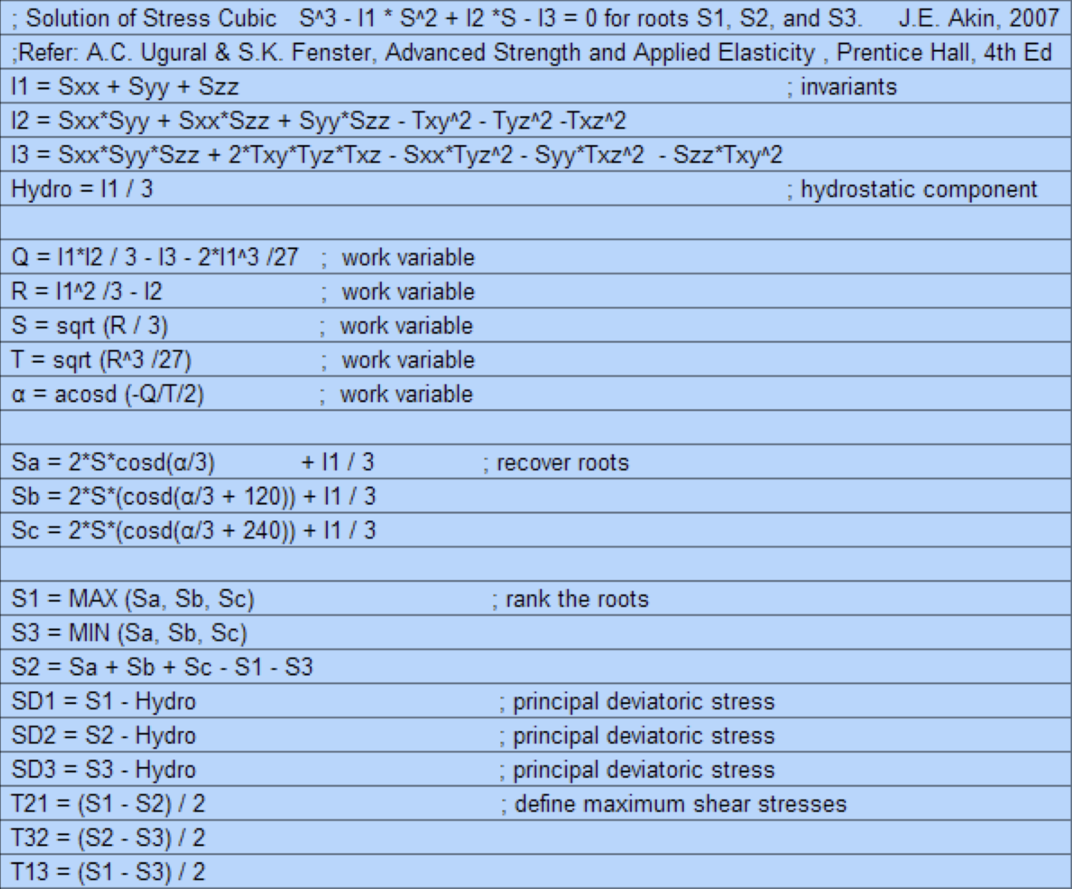

            double *vals = in->GetTuple9(i);   
            double s11 = vals[0], s12 = vals[1], s13 = vals[2];
            double s21 = vals[3], s22 = vals[4], s23 = vals[5];
            double s31 = vals[6], s32 = vals[7], s33 = vals[8];

            // Hydro-static component
            double pressure = (s11 + s22 + s33) / 3.;

            // Deviatoric stress components
            double dev0 = s11 - pressure;
            double dev1 = s22 - pressure;
            double dev2 = s33 - pressure;

            // double invariant0 = dev0 + dev1 + dev2;
            // Second invariant of stress deviator
            double invariant1 = 0.5*(dev0*dev0 + dev1*dev1 + dev2*dev2);
            invariant1 += s12*s12 + s13*s13 + s23*s23;

            // Third invariant of stress deviator
            double invariant2 = -dev0*dev1*dev2;
            invariant2 += -2.0*s12*s13*s23;
            invariant2 +=     dev0*s23*s23;
            invariant2 +=     dev1*s13*s13;
            invariant2 +=     dev2*s12*s12;

            // Cubic roots of the characteristic equation
            // http://mathworld.wolfram.com/CubicFormula.html
            double princ0 = 0.;
            double princ2 = 0.;
            if (invariant1 >= 1e-100)
            {
                double alpha = -0.5*sqrt(27./invariant1)
                                  *invariant2/invariant1;
                if (alpha < 0.)
                    alpha = (alpha < -1. ? -1 : alpha);
                if (alpha > 0.)
                    alpha = (alpha > +1. ? +1 : alpha);

                double angle = acos((double)alpha) / 3.;
                double value = 2.0 * sqrt(invariant1 / 3.);
                princ0 = value*cos(angle);
                // Displace the angle for princ1 (which we don't calculate)
                angle = angle - 2.0*vtkMath::Pi()/3.;
                // Now displace for princ2
                angle = angle + 4.0*vtkMath::Pi()/3.;
                princ2 = value*cos(angle);
            }

            // set the output value

Trace Function: trace() : trace(expr0): Creates a new scalar expression which is everywhere the trace of expr0 which must be a 3x3 tensor. The trace is the sum of the diagonal elements.

Viscous Stress Function: viscous_stress() : viscous_stress(expr0)

Creates a new tensor expression which is everywhere the viscous stress. The key difference between viscous stress and elastic stress (which is the kind of stress many of the other functions here deal with) is that viscous stress is related to the rate of change of deformation whereas elastic stress is related to the amount of deformation. These two are related in the same way velocity and distance are related.

The argument here, expr0 is a vector valued velocity. In addition, the current implementation of this function works only for 2D, structured gridded meshes.

Show/Hide Code for viscous_stress()

    dx[0] = .5 * (px[0] + px[1] - px[2] - px[3]);
    dx[1] = .5 * (px[1] + px[2] - px[3] - px[0]);

    dy[0] = .5 * (py[0] + py[1] - py[2] - py[3]);
    dy[1] = .5 * (py[1] + py[2] - py[3] - py[0]);

    du[0] = .5 * (vx[0] + vx[1] - vx[2] - vx[3]);
    du[1] = .5 * (vx[1] + vx[2] - vx[3] - vx[0]);

    dv[0] = .5 * (vy[0] + vy[1] - vy[2] - vy[3]);
    dv[1] = .5 * (vy[1] + vy[2] - vy[3] - vy[0]);

    div = 1.0 / (dx[0] *dy[1] - dx[1] *dy[0] + tiny);

    dvx[0] = div * (du[0]*dy[1] - du[1] * dy[0]);
    dvx[1] = div * (du[1]*dx[0] - du[0] * dx[1]);

    dvy[0] = div * (dv[0]*dy[1] - dv[1] * dy[0]);
    dvy[1] = div * (dv[1]*dx[0] - dv[0] * dx[1]);

    // create the tensor

    // if rz mesh include extra divergence term
    if( rz_mesh )
    {
        cyl_term = (vy[0] + vy[1] + vy[2] + vy[3]) /
                   (py[0] + py[1] + py[2] + py[3] + tiny);
    }

    // diag terms
    vstress[0] = 1/3.0 * (2.0 * dvx[0] - dvy[1]- cyl_term);
    vstress[4] = 1/3.0 * (2.0 * dvy[1] - dvx[0]- cyl_term);
    vstress[8] = 0.0;
    // other terms
    vstress[1] = 0.5 * (dvy[0]  + dvx[1]);
    vstress[2] = 0.0;
    vstress[5] = 0.0;

    // use symm to fill out remaining terms
    vstress[3] = vstress[1];
    vstress[6] = vstress[2];
    vstress[7] = vstress[5];
}

8.1.3.6. Array Expressions¶

Array Compose Function: array_compose() : array_compose(expr0, expr1, ..., exprN-1): Create a new array expression variable which is everywhere the array composition of its arguments, which all must be scalar type. An array mesh variable is useful when using the label plot or when doing picks and wanting pick values to always return a certain selected set of mesh variables. But, all an array mesh variable really is is a convenient container to hold a group of individual scalar mesh variables. Each argument to the array_compose expression must evaluate to a scalar expression and all of the input expressions must have the same centering. Array variables are collections of scalar variables that are commonly used with certain plots to display the contents of multiple variables simultaneously. For example, the Label plot can display the values in an array variable.

Array Compose With Bins Function: array_compose_with_bins() : array_compose_with_bins(expr0,...,exprN-1,b0,...bn-1 )

This expression combines two related concepts. One is the array concept where a group of individual scalar mesh variables are grouped into an array variable. The other is a set of coordinate values (you can kinda think of as bin boundaries), that should be used by VisIt for certain kinds of operations involving the array variable. If there are N variables in the array, expr0, expr1, and so on, there are N+1 coordinate values (or bin boundaries), b0, b1. When such a variable is picked using one of VisIt’s pick operations, VisIt can display a bar-graph. Each bar in the bar-graph has a height determined by the associated scalar mesh variable (at the picked point) and a width determined by the associated bin-boundaries.

For example, suppose a user had an array variable, foo, composed of 5 scalar mesh variables, a1, a2, a3, a4, and a5 like so…

array_compose_with_bins(a1,a2,a3,a4,a5,0,3.5,10.1,10.7,12,22)

For any given point on a plot, when the user picked foo, there are 5 values returned, the value of each of the 5 scalar variable members of foo. If the user arranged for a pick to return a bar-graph of the variable using the bin-boundaries, the result might look like…

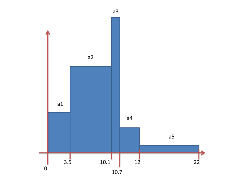
../../_images/new_array_compose_with_bins.png

Fig. 8.4 Bar graph created from picking an array variable created with array_compose_with_bins()

Array Decompose Function: array_decompose() : array_decompose(Arr,Idx): Creates a new scalar expression which is everywhere the scalar member of the array input argument at index Idx (numbered starting from zero).

Array Decompose 2D Function: array_decompose2d() : array_decompose2d(expr0): No description available.

Array Component-wise Division Function: array_componentwise_division() : array_componentwise_division(<Array>,<Divisor>): Return a new array variable which is the old input <Array> variable with each of its components divided by the <Divisor>.

Array Component-wise Product Function: array_componentwise_product() : array_componentwise_product(<Array>,<Multiplier>): Return a new array variable which is the old input <Array> variable with each of its components multiplied by the <Multiplier>.

Array Sum Function: array_sum() : array_sum(<Array>): Return a new scalar variable which is the sum of the <Array> components.

8.1.3.7. Material Expressions¶

Dominant Material Function: dominant_mat() : domimant_mat(<Mesh>): Creates a new scalar expression which is for every mesh cell/zone the material having the largest volume fraction.

Material Error Function: materror() : materror(<Mat>,[Const,Const...])

Creates a new scalar expression which is everywhere the difference in volume fractions as stored in the database and as computed by VisIt’s material interface reconstruction (MIR) algorithm. The <Mat> argument is a material variable from a database and the Const argument is one of the material names as an quoted string or a material number as an integer. If multiple materials are to be selected from the material variable, enclose them in square brackets as a list.

Examples…

materror(materials, 1)
materror(materials, [1,3])
materror(materials, "copper")
materror(materials, ["copper", "steel"])

Material Volume Fractions Function: matvf() : matvf(<Mat>,[Const,Const,...])

Creates a new scalar expression which is everywhere the sum of the volume fraction of the specified materials within the specified material variable. The <Mat> argument is a material variable from a database and the Const argument(s) identify one or more materials within the material variable.

Examples…

matvf(materials, 1)
matvf(materials, [1,3])
matvf(materials, "copper")
matvf(materials, ["copper", "steel"])

NMats Function: nmats() : nmats(<Mat>): Creates a new scalar expression which for each mesh cell/zone is the number of materials in the cell/zone. The <Mat> argument is a material variable from a database.

Specmf Function: specmf() : specmf(<Spec>,<MConst>,[Const,Const,...])

Performs the analogous operation to matvf for species mass fractions. The <Spec> argument is a species variable from a database. The <MConst> argument is a specific material within the species variable. The <Const> argument(s) identify which species within the species variable to select.

Examples:

specmf(species, 1, 1)
specmf(species, "copper", 1)
specmf(species, "copper", [1,3])

Value For Material Function: value_for_material() : value_for_material(<Var>,<Const>): Creates a new scalar expression which is everywhere the material-specific value of the variable specified by <Var> for the material specified by <Const>. If variable specified by <Var> has no material specific values, the values returned from this function will be just the variable’s values.

8.1.3.8. Mesh Expressions¶

Area Function: area() : area(<Mesh>): See the Verdict Manual

cylindrical Function: cylindrical() : cylindrical(<Mesh>): Creates a new vector variable on the mesh which is the cylindrical coordinate tuple (R,theta,Z) of each mesh node.

Cylindrical Radius : cylindrical_radius(<Mesh>): Creates a scalar new variable on the mesh which is the radius component of the cylindrical coordinate (from the Z axis) of each mesh node.

cylindrical theta Function: cylindrical_theta() : cylindrical_theta(<Mesh>): Creates a new scalar variable on the mesh which is the angle component of the cylindrical coordinate (around the Z axis from the +X axis) of each mesh node.

polar radius Function: polar_radius() : polar_radius(<Mesh>): Creates a new scalar variable on the mesh which is the radius component of the polar coordinate of each mesh node.

polar theta Function: polar_theta() : polar_theta(<Mesh>): Creates a new scalar variable on the mesh which is the theta component of the polar coordinate of each mesh node.

polar phi Function: polar_phi() : polar_phi(<Mesh>): Creates a new scalar variable on the mesh which is the phi component of the polar coordinate of each mesh node.

min coord Function: min_coord() : min_coord(expr0): No description available.

max coord Function: max_coord() : max_coord(expr0): No description available.

external node Function: external_node() : external_node(expr0): No description available.

external cell Function: external_cell() : external_cell(expr0): No description available.

Zoneid Function: zoneid() : zoneid(<Mesh>): Return a zone-centered scalar variable where the value for each zone/cell is local index of a zone, staring from zero, within its domain.

Global Zoneid Function: global_zoneid() : global_zoneid(<Mesh>): If global zone ids are specified by the input database, return a zone-centered scalar variable where the value for each zone/cell is the global index of a zone, as specified by the data producer.

Nodeid Function: nodeid() : nodeid(expr0): Return a node-centered scalar variable where the value for each node/vertex/point is local index of a node, staring from zero, within its domain.

Global Nodeid Function: global_nodeid() : global_nodeid(expr0): If global node ids are specified by the input database, return a node-centered scalar variable where the value for each node/vertex/point is the global index of a node, as specified by the data producer.

Volume Function: volume() : volume(<Mesh>): No description available.

Volume2 Function: volume2() : volume2(<Mesh>): No description available.

Revolved Volume Function: revolved_volume() : revolved_volume(<Mesh>): No description available.

Revolved Surface Area Function: revolved_surface_area() : revolved_surface_area(<Mesh>): No description available.

Zone Type Function: zonetype() : zonetype(<Mesh>): Return a zone centered, character valued variable which indicates the shape type of each zone suitable for being used within the label plot. Upper case characters generally denote 3D shapes (e.g. T for tet) while lower case characters denote 2D shapes (e.g. t for triangle).

Zone Type Rank Function: zonetype_rank() : zonetype_rank(<Mesh>): Return a zone centered, integer valued variable which indicates the VTK shape type of each zone. This expression is often useful with the threshold operator to select only certain shapes within the mesh to be displayed.

8.1.3.9. Mesh Quality Expressions¶

VisIt employs the Verdict Mesh Quality Library to support a number of expressions related to computing cell-by-cell mesh quality metrics. The specific definitions of the various mesh quality metrics defined by the Verdict Mesh Quality Library are amply explained in the Verdict Manual. Below, we simply list all the mesh quality metrics and describe in detail only those that are not part of the Verdict Mesh Quality Library

In all cases in the Mesh Quality Expressions, the input argument is a mesh variable from a database and the output is a scalar expression.

Neighbor Function: neighbor() : neighbor(<Mesh>): See the Verdict Manual

Node Degree Function: node_degree() : node_degree(<Mesh>): See the Verdict Manual

degree Function: degree() : degree(expr0): No description available.

Aspect Function: aspect() : aspect(<Mesh>): See the Verdict Manual

Skew Function: skew() : skew(<Mesh>): See the Verdict Manual

Taper Function: taper() : taper(<Mesh>): See the Verdict Manual

Minimum Corner Angle Function: min_corner_angle() : min_corner_angle(<Mesh>): See the Verdict Manual

Maximum Corner Angle Function: max_corner_angle() : max_corner_angle(<Mesh>): See the Verdict Manual

Minimum Edge Length Function: min_edge_length() : min_edge_length(<Mesh>): See the Verdict Manual

Maximum Edge Length Function: max_edge_length() : max_edge_length(<Mesh>): See the Verdict Manual

Minimum Side Volume Function: min_side_volume() : min_side_volume(<Mesh>): See the Verdict Manual

Maximum Side Volume Function: max_side_volume() : max_side_volume(<Mesh>): See the Verdict Manual

Stretch Function: stretch() : stretch(<Mesh>): See the Verdict Manual

Diagonal Ratio Function: diagonal_ratio() : diagonal_ratio(<Mesh>): See the Verdict Manual

Maximum Diagonal Function: max_diagonal() : max_diagonal(<Mesh>): See the Verdict Manual

Minimum Diagonal Function: min_diagonal() : min_diagonal(<Mesh>): See the Verdict Manual

Dimension Function: dimension() : dimension(<Mesh>): See the Verdict Manual

Oddy Function: oddy() : oddy(<Mesh>): See the Verdict Manual

Condition Function: condition() : condition(<Mesh>): See the Verdict Manual

Jacobian Function: jacobian() : jacobian(<Mesh>): See the Verdict Manual

Scaled Jacobian Function: scaled_jacobian() : scaled_jacobian(<Mesh>): See the Verdict Manual

Shear Function: shear() : shear(<Mesh>): See the Verdict Manual

Shape Function: shape() : shape(<Mesh>): See the Verdict Manual

Relative Size Function: relative_size() : relative_size(<Mesh>): See the Verdict Manual

Shape and Size Function: shape_and_size() : shape_and_size(<Mesh>): See the Verdict Manual

Aspect Gamma Function: aspect_gamma() : aspect_gamma(<Mesh>): See the Verdict Manual

Warpage Function: warpage() : warpage(<Mesh>): See the Verdict Manual

Maximum Angle Function: maximum_angle() : maximum_angle(<Mesh>): See the Verdict Manual

Minimum Angle Function: minimum_angle() : minimum_angle(<Mesh>): See the Verdict Manual

Minimum Corner Area Function: min_corner_area() : min_corner_area(<Mesh>): See the Verdict Manual

Minimum Sin Corner Function: min_sin_corner() : min_sin_corner(<Mesh>): See the Verdict Manual

Minimum Sin Corner CW Function: min_sin_corner_cw() : min_sin_corner_cw(<Mesh>): See the Verdict Manual

Face Planarity Function: face_planarity() : face_planarity(<Mesh>): Creates a new expression which is everywhere a measure of how close to planar all the points comprising a face are. This is computed for each face of a cell and the maximum over all faces is selected for each cell. Planarity is measured as the maximum distance from an arbitrary plane defined by the first 3 points of a face of the remaining points of the face. Values closer to zero are better. A triangle face will always have a planarity measure of zero. This mesh quality expression is not part of the Verdict library.

Relative Face Planarity Function: relative_face_planarity() : relative_face_planarity(<Mesh>): Performs the same computation as the face_planarity(), except where each face’s value is normalized by the average edge length of the face.

8.1.3.10. Comparison Expressions¶

Comparing variables defined on the same mesh is often as simple as taking their difference. What about comparing variables when they are defined on different meshes? A common example is taking the difference between results from two runs of the same simulation application. Even if the two runs operate on computationally identical meshes, the fact that each run involves its own instance of that mesh means that as far as VisIt is concerned, they are different meshes.

In order to compose an expression involving variables on different meshes, the first step is to map the variables onto a common mesh. The position-based CMFE function and its friend, the connectivity-based CMFE function, conn_cmfe() are the work-horse methods needed when working with variables from different meshes in the same expression. CMFE is an abbreviation for cross-mesh field evaluation.

The syntax for specifying CMFE expressions can be complicated. Therefore, the GUI supports a wizard to help create them. See the Data-Level Comparisons Wizard for more information. Here, we describe the details of creating CMFE expressions manually.

All of the comparison expressions involve the concepts of a donor variable and a target mesh. The donor variable (e.g. pressure) is the variable to be mapped. The target mesh is the mesh onto which the donor variable is to be mapped. In addition, the term donor mesh refers to the mesh upon which the donor variable is defined.

Position-Based CMFE Function: pos_cmfe() : pos_cmfe(<Donor Variable>,<Target Mesh>,<Fill>)

The pos_cmfe() function performs the mapping assuming the two meshes, that is the <Target Mesh> and the mesh upon which the <Donor Variable> (e.g. the donor mesh) is defined, share only a common spatial (positional) extent. Its friend, the conn_cmfe() function is optimized to perform the mapping when the two meshes are also topologically identical. In other words, their coordinate and connectivity arrays are 1:1. In this case, the mapping can be performed with more efficiency and numerical accuracy. Therefore, when it is possible and makes sense to do so, it is always best to use conn_cmfe().

We’ll describe the arguments to pos_cmfe() working backwards from the last.

The last, <Fill> argument is a numerical constant that VisIt will use to determine the value of the result in places on the target mesh that do not spatially overlap with the mesh of the donor variable. Note that if a value is chosen within the range of the donor variable, it may by difficult to distinguish regions VisIt deemed were non-overlapping. On the other hand, if a value outside the range is chosen, it will effect the range of the mapped variable. A common practice is to choose a value that is an extremum of the donor variable’s range. Another practice is to choose a value that is easily distinguishable and then apply a threshold operator to remove those portions of the result. If the Fill argument is not specified, zero is assumed.

Working backwards, the next argument, is the <Target Mesh>. The <Target Mesh> argument in pos_cmfe() is always interpreted as a mesh within the currently active database. The CMFE expressions are always mapping data from other meshes, possibly in other databases onto the <Target Mesh> which is understood to be in the currently active database. When mapping data between meshes in different databases, the additional information necessary to specify the other database is encoded with a special syntax prepending the Donor Variable argument.

The Donor Variable argument is a string argument of the form:
<PATH-TO-DATABASE-FROM-CWD[SSS]MM:VARNAME>
consisting of the donor variable’s name and up to three pre-pending sub-strings which may be optionally needed to specify…

…the Database (PATH-TO-DATABASE-FROM-CWD) in which the donor variable resides,

…the State Id ([SSS]) from which to take the donor variable,

…the Modality (MM) by which states are identified in the State Id sub-string.

Depending on circumstances, specifying the Donor-Variable argument to the CMFE functions can get cumbersome. For this reason, CMFE expressions are typically created using the Data-Level Comparisons Wizard under the Controls menu. Nonetheless, here we describe the syntax and provide examples for a number of cases of increasing complexity in specifying where the Donor Variable resides.

When the donor variable is in the same database and state as the target mesh, then only the variable’s name is needed. The optional substrings are not. See case A in the examples below.

When the donor variable is in a different database and the databases do not have multiple time states, then only sub-string 1, above, is needed to specify the path to the database in the file system. The path to the database can be specified using either absolute or relative paths. Relative paths are interpreted relative to the current working directory in which the VisIt session was started. See cases B and C in the examples below.

When the donor variable is in a different database and the databases have multiple states, then all 3 sub-strings, above, are required. The State Id substring is a square-bracket enclosed number used to identify which state from which to take the donor variable. The Modality substring is a one- or two-character moniker. The first character indicates whether the number in the the State Id substring is a cycle (c), a time (t), or an index (i). The second character, if present, is a d character to indicate the cycle, time or index is relative (e.g. a delta) to the current state. For example, the substring [200]c means to treat the 200 as a cycle number in the donor database whereas the the substring [-10]id means to treat the -10 as an (i) index (d) delta. So, [200]c would map the donor at cycle 200 to the current cycle of the target and [-10]id would map the donor at the current index minus 10 to the current index of the target. In particular, the string [0]id is needed to create a CMFE that keeps donor and target in lock step. Note that in cases where the donor database does not have an exact match for the specified cycle or time, VisIt will chose the state with the cycle or time which is closest in absolute distance. For the index modality, if there is no exact match for the specified index, an error results. See cases D-I in the examples below.

Note that the relative form of specifying the State Id is needed even when working with different states within the same database. In particular, to create an expression representing a time derivative of a variable in a database, the key insight is to realize it involves mapping a donor variable from one state in the database onto a mesh at another state. In addition, the value in using the relative form of specifying the State Id of the donor variable is that as the current time is changed, the expression properly identifies the different states of the donor variable instead of always mapping a fixed state.

Examples…

# Case A: Donor variable, "pressure" in same database as mesh, "ucdmesh"
# Note that due to a limitation in Expression parsing, the '[0]id:' is
# currently required in the donor variable name as a substitute for
# specifying a file system path to a database file. The syntax '[0]id:'
# means a state index delta of zero within the active database.
pos_cmfe(<[0]id:pressure>,<ucdmesh>,1e+15)

# Case B: Donor variable in a different database using absolute path
pos_cmfe(</var/tmp/foo.silo:pressure>,<ucdmesh>,1e+15)

# Case C: Donor variable in a different database using relative path
pos_cmfe(<foo/bar.silo:pressure>,<ucdmesh>,1e+15)

# Case D: Map "p" from wave.visit at state index=7 onto "mesh"
pos_cmfe(<./wave.visit[7]i:p>, mesh, 1e+15)

# Case E: Map "p" from wave.visit at state index current-1 onto "mesh"
pos_cmfe(<./wave.visit[-1]id:p>, mesh, 1e+15)

# Case F: Map "p" from wave.visit at state with cycle~200 onto "mesh"
pos_cmfe(<./wave.visit[200]c:p>, mesh, 1e+15)

# Case G: Map "p" from wave.visit at state with cycle~cycle(current)-200 onto "mesh"
pos_cmfe(<./wave.visit[-200]id:p>, mesh, 1e+15)

# Case H: Map "p" from wave.visit at state with time~1.4 onto "mesh"
pos_cmfe(<./wave.visit[1.4]t:p>, mesh, 1e+15)

# Case I: Map "p" from wave.visit at state with time~time(current)-0.8 onto "mesh"
pos_cmfe(<./wave.visit[-0.8]td:p>, mesh, 1e+15)

Connectivity-Based CMFE Function: conn_cmfe() : conn_cmfe(<Donor Variable>,<Target Mesh>): The connectivity-based CMFE is an optimized version of pos_cmfe() for cases where the Target Mesh and the mesh of the Donor Variable are topologically and geometrically identical. In such cases, there is no opportunity for the two meshes to fail to overlap perfectly. Thus, there is no need for the third, <Fill> argument. In all other respects, conn_cmfe() performs the same function as pos_cmfe() except that conn_cmfe() assumes that any differences in the coordinates of the two meshes are numerically insignificant to the resulting mapped variable. In other words, differences in the coordinate fields, if they exist, are not incorporated into the resulting mapping.

Curve CMFE Function: curve_cmfe() : curve_cmfe(<Donor Curve>,<Target Curve>): The curve-based CMFE performs the same function as pos_cmfe() except for curves. The arguments specify the Target Curve and Donor Curve and the same syntax rules apply for specifying the Donor Curve as for the Donor Variable in pos_cmfe(). However, if curves represent different spatial extents or different numbers of samples or sample spacing, no attempt is made to unify them.

Symmetric Difference By Point Function: symm_point() : symm_point(<Scalar>,<Fill>,[Px,Py,Pz]): Return a new scalar variable which is the symmetric difference of <Scalar> reflected about the point [Px, Py, Pz]. In 2D, Pz is still required but ignored. The <Fill> argument is a numerical constant that VisIt will use to determine the value of the result in places symmetry about the point doesn’t overlap with the donor mesh. This operation involves both the reflection about the point and taking the difference. If the input <Scalar> is indeed symmetric about the point, the result will be a constant valued variable of zero.

Symmetric Difference By Plane Function: symm_plane() : symm_plane(<Scalar>,<Fill>,[Nx,Ny,Nz,Px,Py,Pz]): Return a new scalar variable which is the symmetric difference of <Scalar> reflected about the plane defined by the point [Px, Py, Pz] and normal [Nx, Ny, Nz]. In 2D, the Nz and Pz arguments are still required but ignored. The <Fill> argument is a numerical constant that VisIt will use to determine the value of the result in places symmetry about the plane doesn’t overlap with the donor mesh. This operation involves both the reflection about the plane and taking the difference. If the input <Scalar> is indeed symmetric about the plane, the result will be a constant valued variable of zero.

Symmetric Difference By Transform Function: symm_transform() : symm_transform(<Scalar>,<Fill>,[T00,T01,T02,...,T22]): Return a new scalar variable which is the symmetric difference of <Scalar> reflected through the 3x3 transformation where each point, [Px,Py,Pz], in the mesh supporting <Scalar> is transformed by the transform coefficients, [T00, T01,...,T22] as shown below. In 2D, all 9 transform coefficients are still required but the last row and column are ignored. The <Fill> argument is a numerical constant that VisIt will use to determine the value of the result in places symmetry through the transform doesn’t overlap with the donor mesh. This operation involves both the transform and taking the difference. If the input <Scalar> is indeed symmetric through the transform, the result will be a constant valued variable of zero.

\[\begin{split}\begin{bmatrix} T_{00} & T_{01} & T_{02} \\ T_{10} & T_{11} & T_{12} \\ T_{20} & T_{21} & T_{22} \end{bmatrix} * \begin{bmatrix} P_{x} \\ P_{y} \\ P_{z} \end{bmatrix} = \begin{bmatrix} T_{00}*P_{x}+T_{01}*P_{y}+T_{02}*P_{z} \\ T_{10}*P_{x}+T_{11}*P_{y}+T_{12}*P_{z} \\ T_{20}*P_{x}+T_{21}*P_{y}+T_{22}*P_{z} \end{bmatrix}\end{split}\]

Evaluate Point Function: eval_point() : eval_point(<Scalar>,<Fill>,[Px,Py,Pz]): Performs only the reflection half of the symm_point() operation. That is, it computes a new scalar variable which is the input <Scalar> reflected through the symmetric point. It does not then take the difference between with the input <Scalar> as symm_point() does.

Evaluate Plane Function: eval_plane() : eval_plane(<Scalar>,<Fill>,[Nx,Ny,Nz,Px,Py,Pz]): Performs only the reflection half of the symm_plane() operation. That is, it computes a new scalar variable which is the input <Scalar> reflected through the symmetric plane. It does not then take the difference between with the input <Scalar> as symm_plane() does.

Evaluate Transform Function: eval_transform() : eval_transform(expr0,<Fill>,[T00,T01,T02...T22]): Performs only the transform half of the symm_transform() operation. That is, it computes a new scalar variable which is the input <Scalar> mapped through the transform. It does not then take the difference between with the input <Scalar> as symm_transform() does.

8.1.3.11. Image Processing Expressions¶

The image processing expressions defined here are not suitable for multi-block data. They do not handle domain boundaries properly even if the input database properly defines suitable layers of ghost zones. They do, however, operate on 2 and 3D data.

conservative smoothing Function: conservative_smoothing() : conservative_smoothing(expr0): No description available.

Mean Filter Function: mean_filter() : mean_filter(<Scalar>,<Int>): Return a filtered version of the input scalar variable using the mean filter of width specified by <Int> argument. By default, the filter width is 3 (3x3). The input scalar must be defined on a structured mesh.

Median Filter Function: median_filter() : median_filter(expr0): Return a filtered version of the input scalar variable using a 3x3 median filter. The input scalar must be defined on a structured mesh.

Abel Inversion Function: abel_inversion() : abel_inversion(expr0): No description available.

8.1.3.12. Miscellaneous Expressions¶

Zonal Constant Function: zonal_constant() : zonal_constant(expr0): Return a scalar, zone-centered field that is everywhere on <Mesh> the constant value <Const>.

Zone Constant Function: zone_constant() : zone_constant(<Mesh>,<Const>): An alias for zonal_constant()

Cell Constant Function: cell_constant() : cell_constant(expr0): An alias for zonal_constant()

Nodal Constant Function: nodal_constant() : nodal_constant(<Mesh>,<Const>): Return a scalar, node-centered field that is everywhere on <Mesh> the constant value <Const>.

Node Constant Function: node_constant() : node_constant(expr0): An alias for nodal_constant()

Point Constant Function: point_constant() : point_constant(expr0): An alias for nodal_constant()

Time Function: time() : time(expr0): Return a constant scalar variable which is everywhere the time of the associated input argument within its time-series.

Cycle Function: cycle() : cycle(expr0): Return an integer constant scalar variable which is everywhere the cycle of the associated input argument within its time-series.

Timestep Function: timestep() : timestep(expr0): Return an integer constant scalar variable which is everywhere the index of the associated input argument within its time-series.

curve domain Function: curve_domain() : curve_domain(expr0): No description available.

curve integrate Function: curve_integrate() : curve_integrate(expr0): No description available.

curve swapxy Function: curve_swapxy() : curve_swapxy(expr0): No description available.

curve Function: curve() : curve(expr0): No description available.

Enumerate Function: enumerate() : enumerate(<Int-Scalar>,<[Int-List]>): Map an integer valued scalar variable to a new set of integer values. If K is the maximum value in the Int-Scalar input argument, the [Int-List] argument must be a square bracketed list of K+1 integer values. Value i in the Int-Scalar input argument is used to index the ith entry in the [Int-List] to produce mapped value.

Map Function: map() : map(<Scalar>,<[Input-Value-List]>,<[Output-Value-List]>, fill_value): A more general form of enumerate() which supports non-integer input scalar variables and input and output maps which are not required to include all values in the input scalar variable. The [Input-Value-List] and [Output-Value-List] must have the same number of entries. A value in the input scalar variable that matches the ith entry in the [Input-Value-List] is mapped to the new value at the ith entry in the [Output-Value-List]. Values that do not match any entry in the [Input-Value-List] are mapped to fill_value, which is -1 by default.

Resample Function: resample() : resample(<Var>,Nx,Ny,Nz): Resample <Var> onto a regular grid defined by taking the X, Y and for 3D, Z spatial extents of the mesh <Var> is defined on and taking Nx samples over the spatial extents in X, Ny samples over the spatial extents in Y, and, for 3D, Nz samples over the spatial extents in Z. Any samples that miss the mesh <Var> is defined on are assigned the value -FLT_MAX. For 2D, the Nz argument is still required but ignored.

Recenter Expression Function : recenter(expr, ["nodal", "zonal", "toggle"]): This function can be used to recenter expr. The second argument is optional and defaults to “toggle” if it is not specified. A value of “toggle” for the second argument means that if expr is node centered, it is recentered to zone centering and if expr is zone centered, it is recentered to node centering. Note that the quotes are required for the second argument. This function is typically used to force a specific centering among the operands of some other expression.

Process Id Function: procid() : procid(<Var>): Return an integer scalar variable which is everywhere the MPI rank associated with each of the blocks of the possibly parallel decomposed mesh upon which <Var> is defined. For serial execution or for parallel execution of a single-block mesh, this will produce a constant zero variable. Otherwise, the values will vary block by block.

Thread Id Function: threadid() : threadid(expr0): Return an integer scalar variable which is everywhere the local thread id associated with each of the blocks of the possibly parallel decomposed mesh upon which <Var> is defined. For non-threaded execution, this will produce a constant zero variable. Otherwise, the values will vary block by block.

isnan Function: isnan() : isnan(expr0): No description available.

q criterion Function: q_criterion() : q_criterion(<gradient(velocity[0])>, <gradient(velocity[1])>, <gradient(velocity[2])>): Generates the Q-criterion value developed by Hunt et. al.. It is based on the observation that, in regions where the Q-criterion is greater than zero, rotation exceeds strain and, in conjunction with a pressure min, indicates the presence of a vortex. The three arguments to the function are gradient vectors of the x-, y-, and z-velocity. The gradient function (see gradient()) can be used to create the gradient vectors.

lambda2 Function: lambda2() : lambda2(<gradient(velocity[0])>, <gradient(velocity[1])>, <gradient(velocity[2])>): Generates the Lambda-2 criterion. It is based on the observation that, in regions where Lambda-2 is less than zero, rotation exceeds strain and, in conjunction with a pressure min, indicates the presence of a vortex. The three arguments to the function are gradient vectors of the x-, y-, and z-velocity. The gradient function (see gradient()) can be used to create the gradient vectors.

mean curvature Function: mean_curvature() : mean_curvature(expr0): No description available.

Gauss Curvature Function: gauss_curvature() : gauss_curvature(expr0): No description available.

agrad Function: agrad() : agrad(expr0): No description available.

key aggregate Function: key_aggregate() : key_aggregate(expr0): No description available.

Laplacian Function: laplacian() : laplacian(expr0): No description available.

rectilinear Laplacian Function: rectilinear_laplacian() : rectilinear_laplacian(expr0): No description available.

conn components Function: conn_components() : conn_components(expr0): No description available.

resrad Function: resrad() : resrad(expr0): No description available.

8.1.3.13. Time Iteration Expressions¶

Average Over Time Function: average_over_time() : average_over_time(<Scalar>,<Start>,<Stop>,<Stride>): Return a new scalar variable in which each zonal or nodal value is the average over the times indicated by Start, Stop and Stride.

Min Over Time Function: min_over_time() : min_over_time(<Scalar>,<Start>,<Stop>,<Stride>): Return a new scalar variable in which each zonal or nodal value is the minimum value the variable, <Scalar>, attained over the times indicated by Start, Stop and Stride.

Max Over Time Function: max_over_time() : max_over_time(<Scalar>,<Start>,<Stop>,<Stride>): Return a new scalar variable in which each zonal or nodal value is the maximum value the variable, <Scalar>, attains over the times indicated by Start, Stop and Stride.

Sum Over Time Function: sum_over_time() : sum_over_time(<Scalar>,<Start>,<Stop>,<Stride>): Return a new scalar variable in which each zonal or nodal value is the sum of the values the variable, <Scalar> attains over the times indicated by Start, Stop and Stride.

First Time When Condition Is True Function: first_time_when_condition_is_true() : first_time_when_condition_is_true(<Cond>,<Fill>,<Start>,<Stop>,<Stride>): Return a new scalar variable in which each zonal or nodal value is the first time (not cycle and not time-index, but floating point time) at which the true/false condition, <Cond> is true. The <Fill> value is used if there is no first time the condition is true.

Last Time When Condition Is True Function: last_time_when_condition_is_true() : last_time_when_condition_is_true(<Cond>,<Fill>,<Start>,<Stop>,<Stride>): Return a new scalar variable in which each zonal or nodal value is the last time (not cycle and not time-index, but floating point time) at which the true/false condition, <Cond> is true. The <Fill> value is used if there is no last time the condition is true.

First Cycle When Condition Is True Function: first_cycle_when_condition_is_true() : first_cycle_when_condition_is_true(<Cond>,<Fill>,<Start>,<Stop>,<Stride>): Return a new integer valued scalar variable in which each zonal or nodal value is the first cycle (not time and not time-index, but integer cycle) at which the true/false condition, <Cond> is true. The <Fill> value is used if there is no first cycle the condition is true.

Last Cycle When Condition Is True Function: last_cycle_when_condition_is_true() : last_cycle_when_condition_is_true(<Cond>,<Fill>,<Start>,<Stop>,<Stride>): Return a new integer valued scalar variable in which each zonal or nodal value is the last cycle (not time and not time-index, but integer cycle) at which the true/false condition, <Cond> is true. The <Fill> value is used if there is no last cycle the condition is true.

First Time Index When Condition Is True Function: first_time_index_when_condition_is_true() : first_time_index_when_condition_is_true(<Cond>,<Fill>,<Start>,<Stop>,<Stride>): Return a new integer valued scalar variable in which each zonal or nodal value is the first time index (not cycle and not time, but integer time-index) at which the true/false condition, <Cond> is true. The <Fill> value is used if there is no first time-index the condition is true.

Last Time Index When Condition Is True Function: last_time_index_when_condition_is_true() : last_time_index_when_condition_is_true(<Cond>,<Fill>,<Start>,<Stop>,<Stride>): Return a new integer valued scalar variable in which each zonal or nodal value is the last time index (not cycle and not time, but integer time-index) at which the true/false condition, <Cond> is true. The <Fill> value is used if there is no last time-index the condition is true.

var when condition is first true Function: var_when_condition_is_first_true() : var_when_condition_is_first_true(expr0): No description available.

var when condition is last true Function: var_when_condition_is_last_true() : var_when_condition_is_last_true(expr0): No description available.

time at minimum Function: time_at_minimum() : time_at_minimum(expr0): No description available.

cycle at minimum Function: cycle_at_minimum() : cycle_at_minimum(expr0): No description available.

time index at minimum Function: time_index_at_minimum() : time_index_at_minimum(expr0): No description available.

value at minimum Function: value_at_minimum() : value_at_minimum(expr0): No description available.

time at maximum Function: time_at_maximum() : time_at_maximum(expr0): No description available.

cycle at maximum Function: cycle_at_maximum() : cycle_at_maximum(expr0): No description available.

time index at maximum Function: time_index_at_maximum() : time_index_at_maximum(expr0): No description available.

value at maximum Function: value_at_maximum() : value_at_maximum(expr0): No description available.

localized compactness Function: localized_compactness() : localized_compactness(expr0): No description available.

merge tree Function: merge_tree() : merge_tree(expr0): No description available.

split tree Function: split_tree() : split_tree(expr0): No description available.

local threshold Function: local_threshold() : local_threshold(expr0): No description available.

python Function: python() : python(expr0): No description available.

relative difference Function: relative_difference() : relative_difference(expr0): No description available.

var skew Function: var_skew() : var_skew(expr0): No description available.

apply data binning Function: apply_data_binning() : apply_data_binning(expr0): No description available.

distance to best fit line Function: distance_to_best_fit_line() : distance_to_best_fit_line(expr0): No description available.

distance to best fit line2 Function: distance_to_best_fit_line2() : distance_to_best_fit_line2(expr0): No description available.

geodesic vector quantize Function: geodesic_vector_quantize() : geodesic_vector_quantize(expr0): No description available.

bin Function: bin() : bin(expr0): No description available.

biggest neighbor Function: biggest_neighbor() : biggest_neighbor(expr0): No description available.

smallest neighbor Function: smallest_neighbor() : smallest_neighbor(expr0): No description available.

neighbor average Function: neighbor_average() : neighbor_average(expr0): No description available.

Displacement Function: displacement() : displacement(expr0): No description available.

8.1.4. Expression Compatibility Gotchas¶

VisIt will allow you to define expressions that it winds up determining to be invalid later when it attempts to execute those expressions. Some common issues are the mixing of incompatible mesh variables in the same expression without the necessary additional functions to make them compatible.

8.1.4.1. Tensor Rank Compatibility¶

For example, what happens if you mix scalar and vector mesh variables in the same expression? VisIt will allow users to define such an expression. But, when it is plotted, the plot will fail.

As an aside, as the user goes back and forth between the Expressions window creating and/or adjusting expression definitions, VisIt makes no attempt to keep track of all the changes made in expressions and automatically update plots as expressions change. Users have to manually clear or delete plots to force VisIt to re-draw plots in which the expressions changed.

If what is really intended was a scalar mesh variable, then users must use one of the expression functions that converts a vector to a scalar such as the magnitude() built-in expression or the array de-reference operator.

8.1.4.2. Centering Compatibility¶

Some variables are zone centered and some are node centered. What happens if a user combines these in an expression? VisIt will default to zone centering for the result. If this is not the desired result, the recenter() expression function should be used, where appropriate, to adjust centering of some of the terms in the expression. Note that ordering of operations will probably be important. For example

node_var + recenter(zone_var)
recenter(zone_var + node_var)

both achieve a node-centered result. But, each expression is subtly (and numerically) different. The first recenter’s zone_var to the nodes and then performs the summation operator at each node. In the second, there is an implied recentering of node_var to the zones first. Then, the summation operator is applied at each zone center and finally the results are recentered back to the nodes. In all likelihood this creates in a numerically lower quality result. The moral is that in a complex series of expressions be sure to take care where you want recentering to occur.

8.1.4.3. Mesh Compatibility¶

In many cases, especially in Silo databases, all the available variables in a database are not always defined on the same mesh. This can complicate matters involving expressions in variables from different meshes.

Just as in the previous two examples of incompatible variables where the solution was to apply some function to make the variables compatible, we have to do the same thing when variables from different meshes are combined in an expression. The key expression functions which enable this are called Cross Mesh Field Evaluation or CMFE expression functions. We will only briefly touch on these here. CMFEs will be discussed in much greater detail elsewhere.

Just as for centering, we have two options when dealing with variables from two different meshes. Each of which involves mapping one of the variables onto the other variable’s mesh using one of the CMFE expression functions.