8.3. X Ray Image Query

8.3.1. Introduction

The X Ray Image Query computes the attenuation and self-emission for radiation passing through an object. The query can be used for EUV radiation and, in some cases, for optical light. The attenuation is used when simulating a radiograph (an xray of a broken bone is a radiograph). If the object is hot enough, it emits xrays and the self-emission is of interest.

The query takes as input a mesh with zone-centered opacities (absorbtivities) and emissivities. The absorbtivity and emissivity variables must be zone-centered and can be either scalar variables (special case) or array variables to support multiple energy groups. The query tracks rays through this mesh, using opacity and emissivity information in each zone to generate an image per radiation energy group. The opacity and emissivity in each zone is a function of radiation energy and rays are tracked for all energies. These rays are regularly spaced in the image plane.

The inputs to the query are usually generated by a computer simulation of the temporal evolution of an object, which records the opacity and emissivity at a set of times. The images produced by the query can be convolved with the spatial, spectral, and temporal response of an (xray) detector in a post-processing step. The simulated data generated using the query can be compared with data recorded during an experiment to see if the simulation is accurate.

The query operates on 2D R-Z meshes and 3D meshes. In the case of 2D R-Z meshes, the mesh is revolved around the Z-axis and the rays are tracked in 3 dimensions.

The query performs the following integration as it traces the rays through the volume.

Show/Hide Code for XRay Image Query

            for (int j = 0 ; j < numBins ; j++)
            {
                double tmp = exp(-a[j] * segLength);
                intensityBins[j] = intensityBins[j] * tmp + e[j] * (1.0 - tmp);
                pathBins[j] = pathBins[j] + a[j] * segLength;
            }

In this code snippet, a represents the absorbtivity, and e represents the emissivity.

If the divide_emis_by_absorb is set, then the following integration is performed.

Show/Hide Code for Absorbtivity-Normalized X Ray Image Query

            for (int j = 0 ; j < numBins ; j++)
            {
                double tmp = exp(-a[j] * segLength);
                intensityBins[j] = intensityBins[j] * tmp + (e[j] / a[j]) * (1.0 - tmp);
                pathBins[j] = pathBins[j] + a[j] * segLength;
            }

When using the divide_emis_by_absorb option, beware of the case where zones have zero absorbtivity. This will lead to NaN intensity results.

When the goal of the query is to generate a radiograph, the user supplies a background intensity (using either background_intensity or background_intensities; see Standard Arguments) and sets the emissivity arrays to zero. The self-emission image produced by the query is then a radiograph.

When the goal of the query is to generate a self-emission image, the emissivities should be non-zero and a background intensity should not be supplied.

Sometimes the goal of an experiment is to generate a radiograph, but the object is hot enough that self-emission might “wash out” the radiograph. In this case, the emissivities should be non-zero and the background intensity should be supplied. The background intensity can then be adjusted until the radiograph is not washed out.

The X Ray Image Query can be used as a part of a larger workflow for simulating X Ray Detectors, namely for the National Ignition Facility. For a discussion of how the query fits into this larger workflow as well as additional detail on our efforts to add Conduit Blueprint output to the query, the following presentation is provided: Supporting Simulated Diagnostics with VisIt’s X Ray Image Query (DOECGF23) Presented at the DOE Computer Graphics Forum 2023.

8.3.2. Query Arguments

The query takes a few different kinds of arguments:

8.3.2.1. Standard Arguments

The standard arguments have to do with the query execution, output, debugging, and passing through metadata.

vars	An array of the names of the absorbtivity and emissivity variables.
background_intensity	The background intensity if ray tracing scalar variables. The default is 0.
background_intensities	The background intensities if ray tracing array variables. The default is 0.
divide_emis_by_absorb	Described above. The default is 0.
image_size	The width and height of the image in pixels. The default is 200 x 200.
debug_ray	The ray index for which to output ray tracing information. The default is -1, which turns it off.
output_ray_bounds	Output the ray bounds as a bounding box in a VTK file. The default is 0 (off). The name of the file is ray_bounds.vtk.
energy_group_bounds	The energy group bounds can be handed off to the query in a list or tuple. The values will appear in the Spatial Extents Mesh in the Blueprint output.

If using the Conduit Output, many of these arguments will appear in the output in a few different places. The vars will show up as abs_var_name and emis_var_name under the Query Parameters section of the Metadata. divide_emis_by_absorb shows up under the Query Parameters section of the Metadata. image_size shows up as num_x_pixels and num_y_pixels under the Query Parameters section of the Metadata. The energy_group_bounds appear under the spatial_coords in the Spatial Extents Meshes.

8.3.2.1.1. Output Filenames and Directories

output_dir		The output directory. The default is “.”
family_files		A flag indicating if the output files should be familied. The default is off. If it is off then the output file is output.ext, where ext is the file extension. If the file exists it will overwrite the file. If it is on, then the output file is outputXXXX.ext, where XXXX is chosen to be the smallest integer not to overwrite any existing files. As of VisIt 3.4, it is recommended to use filename_scheme in lieu of family_files.
filename_scheme		The naming convention for output filenames. This option is available in VisIt 3.4, and is meant to replace the family_files option. If both are provided, filename_scheme will be used.
	“none” or 0	The default. Output filenames will be of the form output.ext, where ext is the file extension. If the filename already exists, VisIt will overwrite it.
	“family” or 1	If on, VisIt will attempt to family output files. Output filenames will be of the form output.XXXX.ext, where XXXX is chosen to be the smallest integer such that the filename is unique.
	“cycle” or 2	VisIt will put cycle information in the filename. Output filenames will be of the form output.cycle_XXXXXX.ext, where XXXXXX is the cycle number. If another file exists with this name, VisIt will overwrite it.

8.3.2.1.2. Output Types

output_type		The format of the image. The default is PNG.
	“bmp” or 0	BMP image format. This is deprecated as of VisIt 3.4.
	“jpeg” or 0 (1 prior to VisIt 3.4)	JPEG image format.
	“png” or 1 (2 prior to VisIt 3.4)	PNG image format.
	“tif” or 2 (3 prior to VisIt 3.4)	TIFF image format.
	“rawfloats” or 3 (4 prior to VisIt 3.4)	File of 32 or 64 bit floating point values in IEEE format.
	“bov” or 4 (5 prior to VisIt 3.4)	BOV (Brick Of Values) format, which consists of a text header file describing a rawfloats file.
	“json” or 5 (6 prior to VisIt 3.4)	Conduit JSON output.
	“hdf5” or 6 (7 prior to VisIt 3.4)	Conduit HDF5 output.
	“yaml” or 7 (8 prior to VisIt 3.4)	Conduit YAML output.

When specifying “bov” or “rawfloats” output, the value can be either 32 or 64 bit floating point values. The number of bits is determined by the number of bits in the data being processed.

When specifying “bov” output, 2 files are created for each variable. One contains the intensity and the other the path_length. The files are named output.XX.bof and output.XX.bov with XX being a sequence number. The intensity variables are first followed by the path_length variables in the sequence. For example, if the input array variables were composed of 2 scalar variables, the files would be named as follows:

• output.00.bof

• output.00.bov - intensity from the first variable of the array variable.

• output.01.bof

• output.01.bov - intensity from the second variable of the array variable.

• output.02.bof

• output.02.bov - path_length from the first variable of the array variable.

• output.03.bof

• output.03.bov - path_length from the second variable of the array variable.

The Conduit output types provide a plethora of extra features; to learn more see Conduit Output.

8.3.2.1.3. Units

Units of various quantities can be passed through the query. None of these values are used in any calculations the query does to arrive at its output; all are optional. These units appear in the Conduit Output in a few different places.

spatial_units	The units of the simulation in the x and y dimensions.
energy_units	The units of the simulation in the z dimension.
abs_units	The units of the absorbtivity variable passed to the query.
emis_units	The units of the emissivity variable passed to the query.
intensity_units	The units of the intensity output.
path_length_info	Metadata describing the path length output.

The spatial_units and energy_units appear in the Spatial Extents Meshes. The abs_units and the emis_units appear in the Query Parameters section of the Metadata. The intensity_units and the path_length_info appear in the Basic Mesh Output and in the 3D Spatial Extents Mesh (Spatial Extents Meshes) under the fields.

8.3.2.2. Camera Specification

The query also takes arguments that specify the orientation of the camera in 3 dimensions. This can take 2 forms. The first is a complete specification that matches the 3D image viewing parameters and the second is a simplified specification that gives limited control over the camera but is easier to use.

8.3.2.2.1. Complete Camera Specification

The complete version consists of:

normal	The view normal. The default is (0., 0., 1.).
focus	The focal point. The default is (0., 0., 0.).
view_up	The up vector. The default is (0., 1., 0.).
view_angle	The view angle. The default is 30. This is only used if perspective projection is enabled.
parallel_scale	The parallel scale, or view height. The default is 0.5.
view_width	The view width. The default is 0.5. If this argument is not specified, the query will assume pixels are to be square, and it will use the specified image_size and the parallel_scale to calculate the correct view_width. If this argument is specified, the query may produce results with non-square pixels.
near_plane	The near clipping plane. The default is -0.5.
far_plane	The far clipping plane. The default is 0.5.
image_pan	The image pan in the X and Y directions. The default is (0., 0.).
image_zoom	The absolute image zoom factor. The default is 1. A value of 2. zooms the image closer by scaling the image by a factor of 2 in the X and Y directions. A value of 0.5 zooms the image further away by scaling the image by a factor of 0.5 in the X and Y directions.
perspective	Flag indicating if doing a parallel or perspective projection. 0 indicates parallel projection. 1 indicates perspective projection.

If any of the above properties are specified in the parameters, the query will use the complete version and disregard all arguments pertaining to the simplified version.

When a Conduit Blueprint output type is specified, these parameters will appear in the metadata. See View Parameters for more information.

8.3.2.2.2. Simplified Camera Specification

The simplified version consists of:

width	The width of the image in physical space. The default is 1.0.
height	The height of the image in physical space. The default is 1.0.
origin	The point in 3D corresponding to the center of the image.
theta phi	The orientation angles. The default is 0. 0. and is looking down the Z axis. Theta moves around the Y axis toward the X axis. Phi moves around the Z axis. When looking at an R-Z mesh, phi has no effect because of symmetry.
up_vector	The up vector.

During execution, the simplified camera specification parameters are converted to the complete ones.

8.3.2.3. Calling the Query

There are a couple ways to call the X Ray Image Query, each with their own nuances.

The first is the standard way of calling the query, by using a dictionary to store the arguments. This way is recommended. Here is an example:

params = dict()
params["image_size"] = (400, 300)
params["output_type"] = "hdf5"
params["focus"] = (0., 2.5, 10.)
params["perspective"] = 1
params["near_plane"] = -25.
params["far_plane"] = 25.
params["vars"] = ("d", "p")
params["parallel_scale"] = 10.
Query("XRay Image", params)

Of course, one could use this to set up the parameters instead:

params = GetQueryParameters("XRay Image")

The default arguments to the query will be provided here, containing the Complete Camera Specification and not the Simplified Camera Specification arguments. To use the Simplified Camera Specification arguments, one must specify them manually and not specify any arguments from the Complete Camera Specification.

The second way to call the query is the old style of argument passing:

Query("XRay Image",
   output_type,
   output_dir,
   divide_emis_by_absorb,
   origin_x,
   origin_y,
   origin_z,
   theta,
   phi,
   width,
   height,
   image_size_x,
   image_size_y,
   vars)

# An example
Query("XRay Image", "hdf5", ".", 1, 0.0, 2.5, 10.0, 0, 0, 10., 10., 400, 300, ("d", "p"))

This way of calling the query exclusively makes use of the Simplified Camera Specification.

8.3.3. Examples

Let’s look at some examples, starting with some simulated x rays using curv2d.silo, which contains a 2D R-Z mesh. Here is a pseudocolor plot of the data.

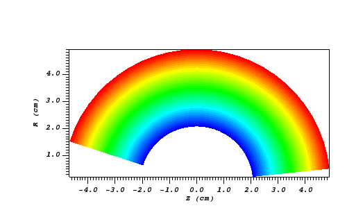
Fig. 8.10 The 2D R-Z data.

Now we will show the Python code to generate a simulated x ray looking down the Z Axis and the resulting image.

params = GetQueryParameters("XRay Image")
params['image_size'] = (300, 300)
params['divide_emis_by_absorb'] = 1
params['width'] = 10.
params['height'] = 10.
params['vars'] = ("d", "p")
Query("XRay Image", params)

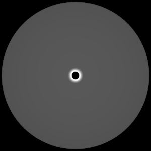
Fig. 8.11 The resulting x ray image.

Here is the Python code to generate the same image but looking at it from the side.

params = GetQueryParameters("XRay Image")
params['image_size'] = (300, 300)
params['divide_emis_by_absorb'] = 1
params['width'] = 10.
params['height'] = 10.
params['theta'] = 90.
params['phi'] = 0.
params['vars'] = ("d", "p")
Query("XRay Image", params)

Fig. 8.12 The resulting x ray image.

Here is the same Python code with the addition of an origin that moves the image down and to the right by 1.

params = GetQueryParameters("XRay Image")
params['image_size'] = (300, 300)
params['divide_emis_by_absorb'] = 1
params['width'] = 10.
params['height'] = 10.
params['theta'] = 90.
params['phi'] = 0.
params['origin'] = (0., 1., 1.)
params['vars'] = ("d", "p")
Query("XRay Image", params)

Fig. 8.13 The resulting x ray image.

Now we will switch to a 3D example using globe.silo. Globe.silo is an unstructured mesh consisting of tetrahedra, pyramids, prisms and hexahedra forming a globe. Here is an image of the tetrahedra at the center of the globe that form 2 cones.

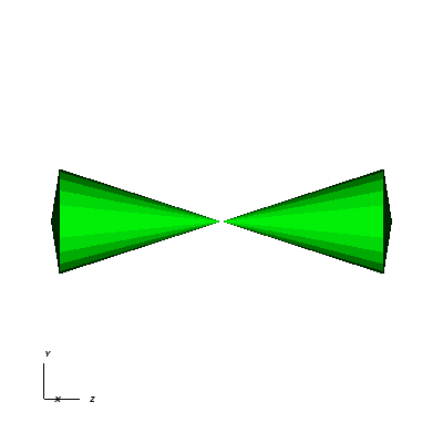
Fig. 8.14 The tetrahedra at the center of the globe.

Here is the Python code for generating an x ray image from the same orientation. Note that we have defined some expressions so that the x ray image shows some variation.

DefineScalarExpression("u1", 'recenter(((u+10.)*0.01), "zonal")')
DefineScalarExpression("v1", 'recenter(((v+10.)*0.01*matvf(mat1,1)), "zonal")')
DefineScalarExpression("v2", 'recenter(((v+10.)*0.01*matvf(mat1,2)), "zonal")')
DefineScalarExpression("v3", 'recenter(((v+10.)*0.01*matvf(mat1,3)), "zonal")')
DefineScalarExpression("v4", 'recenter(((v+10.)*0.01*matvf(mat1,4)), "zonal")')
DefineScalarExpression("w1", 'recenter(((w+10.)*0.01), "zonal")')

params = GetQueryParameters("XRay Image")
params['image_size'] = (300, 300)
params['divide_emis_by_absorb'] = 1
params['width'] = 4.
params['height'] = 4.
params['theta'] = 90.
params['phi'] = 0.
params['vars'] = ("w1", "v1")
Query("XRay Image", params)

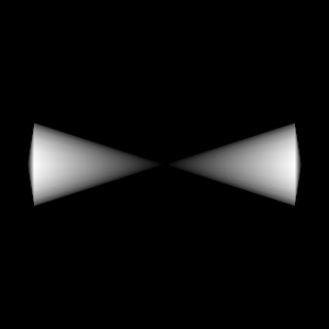
Fig. 8.15 The resulting x ray image.

Now we will look at the pyramids in the center of the globe.

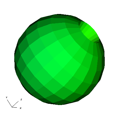
Fig. 8.16 The pyramids at the center of the globe.

Here is the Python code for generating an x ray image from the same orientation using the full view specification. The view specification was merely copied from the 3D tab on the View window.

params = dict(output_type="png")
params['image_size'] = (300, 300)
params['divide_emis_by_absorb'] = 1
params['focus'] = (0., 0., 0.)
params['view_up'] = (-0.0651, 0.775, 0.628)
params['normal'] = (-0.840, -0.383, 0.385)
params['view_angle'] = 30.
params['parallel_scale'] = 17.3205
params['near_plane'] = -34.641
params['far_plane'] = 34.641
params['image_pan'] = (0., 0.)
params['image_zoom'] = 8
params['perspective'] = 0
params['vars'] = ("w1", "v2")
Query("XRay Image", params)

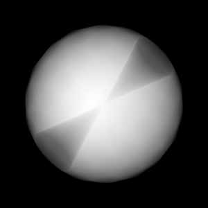
Fig. 8.17 The resulting x ray image.

The next example illustrates use of one of the Conduit Output types.

# A test file
OpenDatabase("testdata/silo_hdf5_test_data/curv3d.silo")

AddPlot("Pseudocolor", "d")
DrawPlots()

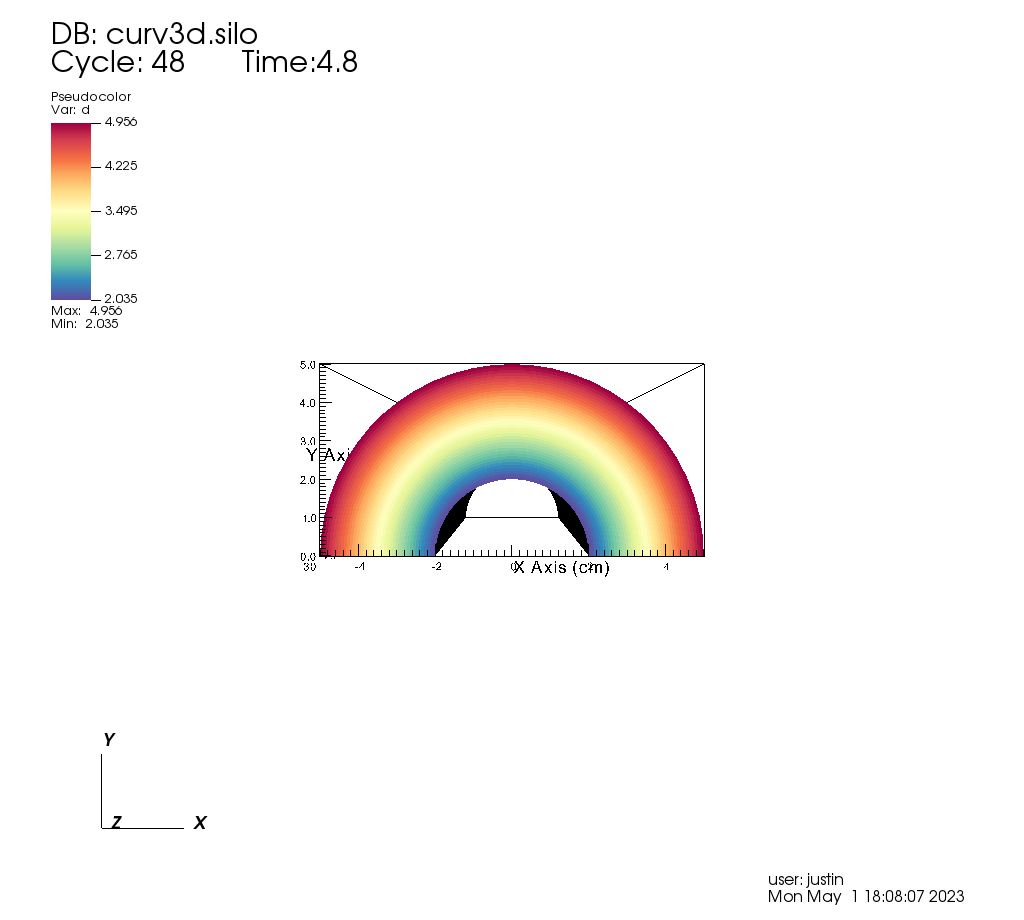
Fig. 8.18 Our input mesh.

We call the query as usual, although there are a few extra arguments we can provide that are used for generating the Conduit output in particular.

params = dict()
params["image_size"] = (400, 300)
params["output_type"] = "hdf5"
params["focus"] = (0., 2.5, 10.)
params["perspective"] = 1
params["near_plane"] = -25.
params["far_plane"] = 25.
params["vars"] = ("d", "p")
params["parallel_scale"] = 10.

# ENERGY GROUP BOUNDS
params["energy_group_bounds"] = [2.7, 6.2]

# UNITS
params["spatial_units"] = "cm"
params["energy_units"] = "kev"
params["abs_units"] = "cm^2/g"
params["emis_units"] = "GJ/cm^2/ster/ns/keV"
params["intensity_units"] = "intensity units"
params["path_length_info"] = "path length metadata"

Query("XRay Image", params)

To look at the raw data from the query, we run this code:

import conduit
xrayout = conduit.Node()

conduit.relay.io.blueprint.load_mesh(xrayout, "output.root")

print(xrayout["domain_000000"])

This yields the following data overview. See Introspecting with Python for a deeper dive into viewing and extracting the raw data from the Conduit Output.

state:
  time: 4.8
  cycle: 48
  xray_view:
    normal:
      x: 0.0
      y: 0.0
      z: 1.0
    focus:
      x: 0.0
      y: 2.5
      z: 10.0
    view_up:
      x: 0.0
      y: 1.0
      z: 0.0
    view_angle: 30.0
    ... ( skipped 6 children )
    image_zoom: 1.0
    perspective: 1
    perspective_str: "perspective"
  xray_query:
    divide_emis_by_absorb: 0
    divide_emis_by_absorb_str: "no"
    num_x_pixels: 400
    num_y_pixels: 300
    ... ( skipped 2 children )
    emis_var_name: "pa"
    abs_units: "cm^2/g"
    emis_units: "GJ/cm^2/ster/ns/keV"
  xray_data:
    detector_width: 8.80338743415454
    detector_height: 6.60254037884486
    intensity_max: 1.96578788757324
    intensity_min: 0.0
    path_length_max: 519.428039550781
    path_length_min: 0.0
    image_topo_order_of_domain_variables: "xyz"
  domain_id: 0
coordsets:
  image_coords:
    type: "rectilinear"
    values:
      x: [0, 1, 2, ..., 399, 400]
      y: [0, 1, 2, ..., 299, 300]
      z: [0, 1, 2, 3, 4]
    labels:
      x: "width"
      y: "height"
      z: "energy_group"
    units:
      x: "pixels"
      y: "pixels"
      z: "bins"
  spatial_coords:
    type: "rectilinear"
    values:
      x: [0.0, 0.0220084685853863, 0.0440169371707727, ..., 8.78137896556915, 8.80338743415454]
      y: [0.0, 0.0220084679294829, 0.0440169358589658, ..., 6.58053191091538, 6.60254037884486]
      z: [0.0, 1.0, 2.0, 3.0, 4.0]
    info: "Energy group bounds size mismatch: provided 7 bounds, but 5 in query results."
    units:
      x: "cm"
      y: "cm"
      z: "kev"
    labels:
      x: "width"
      y: "height"
      z: "energy_group"
  spatial_energy_reduced_coords:
    type: "rectilinear"
    values:
      x: [0.0, 0.0220084685853863, 0.0440169371707727, ..., 8.78137896556915, 8.80338743415454]
      y: [0.0, 0.0220084679294829, 0.0440169358589658, ..., 6.58053191091538, 6.60254037884486]
    units:
      x: "cm"
      y: "cm"
    labels:
      x: "width"
      y: "height"
  spectra_coords:
    type: "rectilinear"
    values:
      x: [0.0, 1.0, 2.0, 3.0, 4.0]
    units:
      x: "kev"
    labels:
      x: "energy_group"
    info: "Energy group bounds size mismatch: provided 7 bounds, but 5 in query results."
  ... ( skipped 2 children )
  far_plane_coords:
    type: "explicit"
    values:
      x: [22.264973744318, -22.264973744318, -22.264973744318, 22.264973744318]
      y: [-14.1987298105776, -14.1987298105776, 19.1987298105776, 19.1987298105776]
      z: [35.0, 35.0, 35.0, 35.0]
  ray_corners_coords:
    type: "explicit"
    values:
      x: [4.40169371707727, 22.264973744318, -4.40169371707727, ..., 4.40169371707727, 22.264973744318]
      y: [-0.801270189422432, -14.1987298105776, -0.801270189422432, ..., 5.80127018942243, 19.1987298105776]
      z: [-15.0, 35.0, -15.0, ..., -15.0, 35.0]
  ray_coords:
    type: "explicit"
    values:
      x: [-4.39068948278457, -4.39068948278457, -4.39068948278457, ..., 22.2093113099572, 22.2093113099572]
      y: [-0.790265955457691, -0.768257487528208, -0.746249019598725, ..., 19.0317425124718, 19.1430673778756]
      z: [-15.0, -15.0, -15.0, ..., 35.0, 35.0]
topologies:
  image_topo:
    coordset: "image_coords"
    type: "rectilinear"
  spatial_topo:
    coordset: "spatial_coords"
    type: "rectilinear"
  spatial_energy_reduced_topo:
    coordset: "spatial_energy_reduced_coords"
    type: "rectilinear"
  spectra_topo:
    coordset: "spectra_coords"
    type: "rectilinear"
  ... ( skipped 2 children )
  far_plane_topo:
    type: "unstructured"
    coordset: "far_plane_coords"
    elements:
      shape: "quad"
      connectivity: [0, 1, 2, 3]
  ray_corners_topo:
    type: "unstructured"
    coordset: "ray_corners_coords"
    elements:
      shape: "line"
      connectivity: [0, 1, 2, ..., 6, 7]
  ray_topo:
    type: "unstructured"
    coordset: "ray_coords"
    elements:
      shape: "line"
      connectivity: [0, 120000, 1, ..., 119999, 239999]
fields:
  intensities:
    topology: "image_topo"
    association: "element"
    units: "intensity units"
    values: [0.0, 0.0, 0.0, ..., 0.0, 0.0]
    strides: [1, 400, 120000]
  path_length:
    topology: "image_topo"
    association: "element"
    units: "path length metadata"
    values: [0.0, 0.0, 0.0, ..., 0.0, 0.0]
    strides: [1, 400, 120000]
  intensities_spatial:
    topology: "spatial_topo"
    association: "element"
    units: "intensity units"
    values: [0.0, 0.0, 0.0, ..., 0.0, 0.0]
    strides: [1, 400, 120000]
  path_length_spatial:
    topology: "spatial_topo"
    association: "element"
    units: "path length metadata"
    values: [0.0, 0.0, 0.0, ..., 0.0, 0.0]
    strides: [1, 400, 120000]
  ... ( skipped 6 children )
  far_plane_field:
    topology: "far_plane_topo"
    association: "element"
    volume_dependent: "false"
    values: 0.0
  ray_corners_field:
    topology: "ray_corners_topo"
    association: "element"
    volume_dependent: "false"
    values: [0.0, 0.0, 0.0, 0.0]
  ray_field:
    topology: "ray_topo"
    association: "element"
    volume_dependent: "false"
    values: [0.0, 1.0, 2.0, ..., 119998.0, 119999.0]

The next thing we may want to do is to visualize an x ray image using VisIt. The Visualizing with VisIt section goes into more detail on this subject, so for now we will only visualize the Basic Mesh Output.

# Have VisIt open the Conduit output from the query
OpenDatabase("output.root")

# Give ourselves a clean slate for ensuing visualizations
DeleteAllPlots()

# Add a pseudocolor plot of the intensities
AddPlot("Pseudocolor", "mesh_image_topo/intensities")
DrawPlots()

# Change the color table to be xray
PseudocolorAtts = PseudocolorAttributes()
PseudocolorAtts.colorTableName = "xray"
SetPlotOptions(PseudocolorAtts)

Running this code yields the following image:

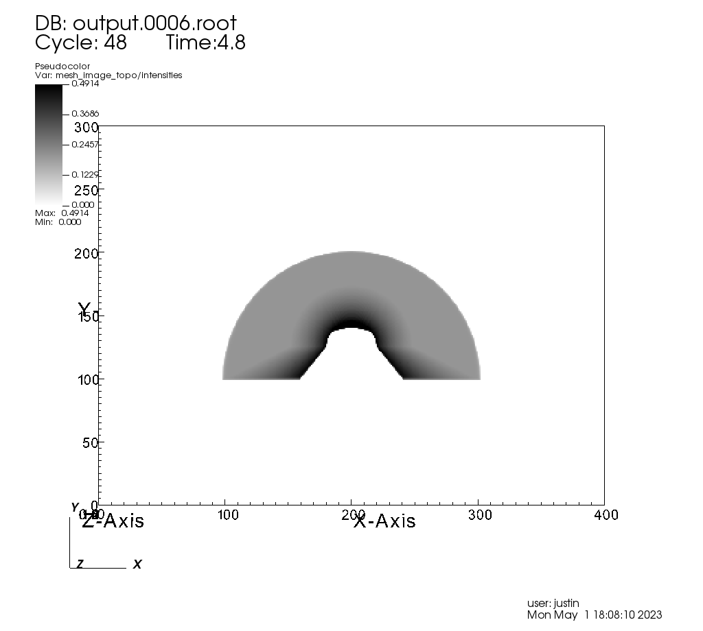
Fig. 8.19 The resulting x ray image, visualized using VisIt.

8.3.4. Conduit Output

The Conduit output types (see Output Types for more information) provide advantages over the other output types and include additional metadata and topologies. These output types were added in VisIt 3.3.0, and many of the features discussed here have been added since then.

8.3.4.1. Why Conduit Output?

Conduit Blueprint output types were added to the X Ray Image Query primarily to facilitate usability and convenience. Before Conduit Blueprint formats were available as output types, the X Ray Image Query would often produce large numbers of output files, particularly when using the BOV or rawfloats output type, which was a popular choice because it provided the raw data. For example, ray tracing 60 energy groups would generate 120 BOV files (one for intensities and one for path lengths for each energy group). These files lack important context and metadata about the details of the ray trace setup. The large number of these files and the inability to control where they were saved led to lots of external data management issues that our users were unfortunately saddled with. Alternatively, users could choose one of the image file output types to generate a picture or pictures. But, without additional post-processing, it was impossible to have both, unless the query was run twice.

We added Conduit Blueprint output as an option to address these problems. Instead of many files coming out of the query, only one comes out. This single output file presents the query output in multiple ways using well-described meshes. We also provide three supported Conduit output types: HDF5, YAML, and JSON. The latter two are useful as they are human-readable options. Instead of having to choose between getting out raw data or getting out an image, Conduit Blueprint provides the best of both worlds. All of the meshes provided in the output can be easily plotted in VisIt (see Visualizing with VisIt), and everything in the output (raw intensities and path lengths data, mesh data, metadata, etc.) can be digested in Python using Conduit’s Python API (see Introspecting with Python).

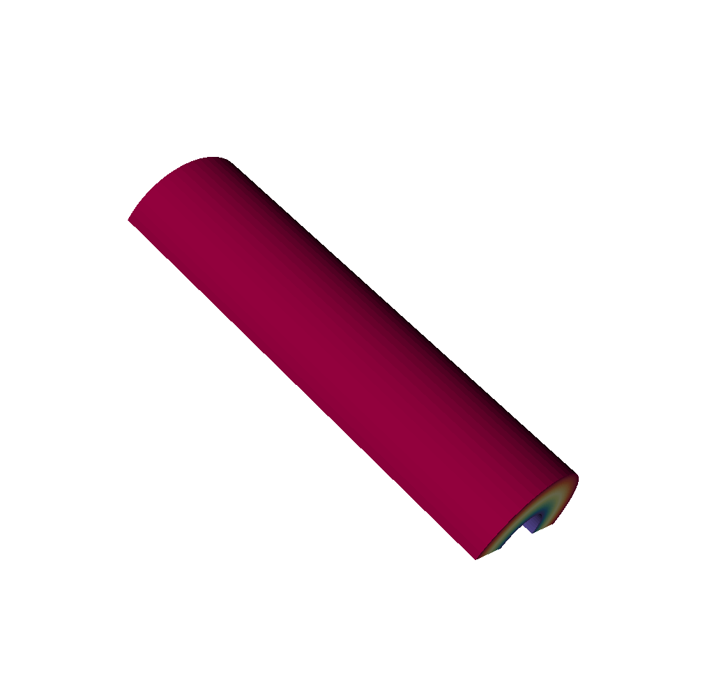
Fig. 8.20 An input mesh.

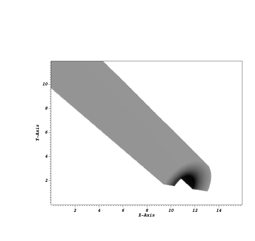
Fig. 8.21 The resulting x ray image from Conduit Blueprint output, visualized by plotting with VisIt.

We have opted to enrich the Blueprint output (see Basic Mesh Output) with extensive metadata (see Metadata) as well as additional meshes (see Imaging Planes and Rays Meshes, Spatial Extents Meshes, and 1D Spectra Curves) to provide extra context and information to the user. These additions should make it easier to troubleshoot unexpected results, make sense of the query output, and pass important information through the query. Blueprint makes it simple to put all of this information into one file, and just as simple to read that information back out and/or visualize.

One of the main reasons for adding the Conduit output was to make it far easier to troubleshoot strange query results. See the Troubleshooting section to see a few examples of the kinds of questions the Conduit output can be used to answer.

8.3.4.2. Overview of Output

So what is actually in the Blueprint output? The Blueprint output provides multiple Blueprint meshes, which are each in turn comprised of a coordinate set, a topology, and fields. These all live within a Conduit tree, along with metadata. Using Conduit allows us to package everything in one place for ease of use.

To extract this data with Python, see Getting a General Overview of the Output. Here is a simplified representation of a Conduit tree that is output from the Query:

state:
  time: 4.8
  cycle: 48
  xray_view:
    ...
  xray_query:
    ...
  xray_data:
    ...
  domain_id: 0
coordsets:
  image_coords:
    ...
  spatial_coords:
    ...
  spatial_energy_reduced_coords:
    ...
  spectra_coords:
    ...
  near_plane_coords:
    ...
  view_plane_coords:
    ...
  far_plane_coords:
    ...
  ray_corners_coords:
    ...
  ray_coords:
    ...
topologies:
  image_topo:
    ...
  spatial_topo:
    ...
  spatial_energy_reduced_topo:
    ...
  spectra_topo:
    ...
  near_plane_topo:
    ...
  view_plane_topo:
    ...
  far_plane_topo:
    ...
  ray_corners_topo:
    ...
  ray_topo:
    ...
fields:
  intensities:
    ...
  path_length:
    ...
  intensities_spatial:
    ...
  path_length_spatial:
    ...
  intensities_spatial_energy_reduced:
    ...
  path_length_spatial_energy_reduced:
    ...
  intensities_spectra:
    ...
  path_length_spectra:
    ...
  near_plane_field:
    ...
  view_plane_field:
    ...
  far_plane_field:
    ...
  ray_corners_field:
    ...
  ray_field:
    ...

There are multiple Blueprint meshes stored in this tree, as well as extensive metadata. Each piece of the Conduit output will be covered in more detail in ensuing parts of the documentation. To learn more about what lives under the state branch, see the Metadata section. To learn more about the coordinate sets, topologies, and fields, see the Basic Mesh Output, Imaging Planes and Rays Meshes, Spatial Extents Meshes, and 1D Spectra Curves sections. To extract this data with Python, see Getting a General Overview of the Output.

8.3.4.2.1. Basic Mesh Output

The most important piece of the Blueprint output is the actual ray trace result. We have taken the image data that comes out of the query and packaged it into a single Blueprint mesh.

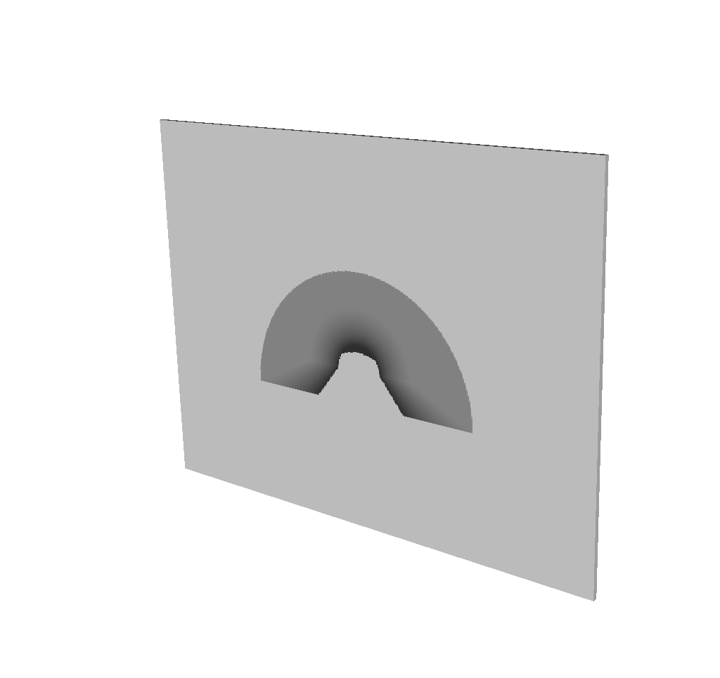
Fig. 8.22 The basic mesh output visualized using VisIt.

To visualize this mesh with VisIt, see Visualizing the Basic Mesh Output. To extract this mesh data with Python, see Accessing the Basic Mesh Output Data. The following is the example from Overview of Output, but with the Blueprint mesh representing the query result fully realized:

state:
  time: 4.8
  cycle: 48
  xray_view:
    ...
  xray_query:
    ...
  xray_data:
    ...
  domain_id: 0
coordsets:
  image_coords:
    type: "rectilinear"
    values:
      x: [0, 1, 2, ..., 399, 400]
      y: [0, 1, 2, ..., 299, 300]
      z: [0, 1]
    labels:
      x: "width"
      y: "height"
      z: "energy_group"
    units:
      x: "pixels"
      y: "pixels"
      z: "bins"
  spatial_coords:
    ...
  spatial_energy_reduced_coords:
    ...
  spectra_coords:
    ...
  near_plane_coords:
    ...
  view_plane_coords:
    ...
  far_plane_coords:
    ...
  ray_corners_coords:
    ...
  ray_coords:
    ...
topologies:
  image_topo:
    coordset: "image_coords"
    type: "rectilinear"
  spatial_topo:
    ...
  spatial_energy_reduced_topo:
    ...
  spectra_topo:
    ...
  near_plane_topo:
    ...
  view_plane_topo:
    ...
  far_plane_topo:
    ...
  ray_corners_topo:
    ...
  ray_topo:
    ...
fields:
  intensities:
    topology: "image_topo"
    association: "element"
    units: "intensity units"
    values: [0.281004697084427, 0.281836241483688, 0.282898783683777, ..., 0.0, 0.0]
    strides: [1, 400, 120000]
  path_length:
    topology: "image_topo"
    association: "element"
    units: "path length metadata"
    values: [2.46405696868896, 2.45119333267212, 2.43822622299194, ..., 0.0, 0.0]
    strides: [1, 400, 120000]
  intensities_spatial:
    ...
  path_length_spatial:
    ...
  intensities_spatial_energy_reduced:
    ...
  path_length_spatial_energy_reduced:
    ...
  intensities_spectra:
    ...
  path_length_spectra:
    ...
  near_plane_field:
    ...
  view_plane_field:
    ...
  far_plane_field:
    ...
  ray_corners_field:
    ...
  ray_field:
    ...

The 3 constituent parts of the Blueprint mesh output are the coordinate set, image_coords, the topology, image_topo, and the fields, intensities and path_length.

The image_coords represent the x and y coordinates of the 2D image, and the z dimension represents the energy group bounds. In the case of multiple energy groups, previously, the query would have output multiple images, one for each pair of energy group bounds. In the Blueprint output, this is simplified; rather than outputting multiple files, each containing one image, we have opted to “stack” the resulting images on top of one another. This is why the Blueprint output is a 3D mesh; this way, it can account for multiple energy groups, and place resulting images one on top of another. Also included in the image_coords are labels and units for disambiguation purposes.

The image_topo exists to tell Blueprint that the rectilinear coordinate data stored in image_coords can be interpreted as a rectilinear grid.

The fields, intensities and path_length, can be thought of as containers for the actual image data. This image data is stored in 1-dimensional arrays; for information on reshaping those into 3-dimensions see the following from the Troubleshooting section: The fields in the Conduit Output are 1D. How can I reshape them to be 3D? Each field also includes units. For path length, the units entry is just a way of including metadata or information about the path length, since path length is unitless.

To visualize this mesh with VisIt, see Visualizing the Basic Mesh Output. To extract this mesh data with Python, see Accessing the Basic Mesh Output Data.

8.3.4.2.2. Metadata

The Conduit output types (see Output Types for more information) come packaged with metadata in addition to Blueprint-conforming mesh data. The ability to send this metadata alongside the output mesh (and other data) is one of the advantages of using Conduit for outputs from the query. We hope this metadata helps to make it clear exactly what the query is doing, what information it has available to it, and what the output might look like. To extract the metadata from the Blueprint output, see Accessing the Metadata.

Metadata is stored under the state Node in the resulting Conduit tree. See the example below, which is taken from the example in Overview of Output, but this time with only the metadata fully realized:

state:
  time: 4.8
  cycle: 48
  xray_view:
    normal:
      x: 0.0
      y: 0.0
      z: 1.0
    focus:
      x: 0.0
      y: 2.5
      z: 10.0
    view_up:
      x: 0.0
      y: 1.0
      z: 0.0
    view_angle: 30.0
    parallel_scale: 5.0
    view_width: 6.667
    non_square_pixels: "no"
    near_plane: -50.0
    far_plane: 50.0
    image_pan:
      x: 0.0
      y: 0.0
    image_zoom: 1.0
    perspective: 1
    perspective_str: "perspective"
  xray_query:
    divide_emis_by_absorb: 0
    divide_emis_by_absorb_str: "no"
    num_x_pixels: 400
    num_y_pixels: 300
    num_bins: 1
    abs_var_name: "d"
    emis_var_name: "p"
    abs_units: "cm^2/g"
    emis_units: "GJ/cm^2/ster/ns/keV"
  xray_data:
    detector_width: 22.3932263237838
    detector_height: 16.7949192423103
    intensity_max: 0.491446971893311
    intensity_min: 0.0
    path_length_max: 120.815788269043
    path_length_min: 0.0
    image_topo_order_of_domain_variables: "xyz"
  domain_id: 0
coordsets:
  ...
topologies:
  ...
fields:
  ...

There are three top-level items: time, cycle, and domain_id. The fact that the domain_id is present is a side effect of Conduit; all of the output data is single domain and this value has nothing to do with the query. In addition to the top level items, there are three categories of metadata: View Parameters, Query Parameters, and Other Metadata. The following subsections discuss each of these categories in more detail.

8.3.4.2.2.1. View Parameters

View parameters can be found under “state/xray_view”. This metadata represents the view-related values that were used in the x ray image query calculations. Remember from the section on Camera Specification options that if the Simplified Camera Specification is used, the parameters are converted to the Complete Camera Specification during execution. Hence the values output here correspond to those in the Complete Camera Specification, as these are the values that were actually used by the query when calculating results. The following is included:

normal	The x, y, and z components represent the view normal vector that was used in the calculations.
focus	The x, y, and z components represent the focal point that was used in the calculations.
view_up	The x, y, and z components represent the up vector that was used in the calculations.
view_angle	The view angle, only used in the calculations if perspective projection was enabled.
parallel_scale	The parallel scale, or view height, that was used in the calculations.
view_width	The view width that was used in the calculations.
non_square_pixels	“yes” means that the output is using non-square pixels, meaning that a view width was specified in the camera setup.
near_plane	The near plane that was used in the calculations.
far_plane	The far plane that was used in the calculations.
image_pan	The x and y components represent the image pan that was used in the calculations.
image_zoom	The absolute image zoom factor that was used in the calculations.
perspective	A flag indicating if parallel or perspective projection was used. 0 indicates parallel projection and 1 indicates perspective projection.
perspective_str	A String representation of the perspective parameter. See above for more information.

An example:

xray_view:
  normal:
    x: 0.0
    y: 0.0
    z: 1.0
  focus:
    x: 0.0
    y: 2.5
    z: 10.0
  view_up:
    x: 0.0
    y: 1.0
    z: 0.0
  view_angle: 30.0
  parallel_scale: 5.0
  view_width: 5.0
  non_square_pixels: "no"
  near_plane: -50.0
  far_plane: 50.0
  image_pan:
    x: 0.0
    y: 0.0
  image_zoom: 1.0
  perspective: 1
  perspective_str: "perspective"

To extract this metadata from the Blueprint output, see Accessing the Metadata.

8.3.4.2.2.2. Query Parameters

Query parameters can be found under “state/xray_query”. This metadata represents the query-related values that were used in the x ray image query calculations. This data is available as of VisIt 3.3.2. The following is included:

divide_emis_by_absorb	A flag indicating if emissivity was divided by absorbtivity in the calculations. More details can be found above.
divide_emis_by_absorb_str	A String representation of the divide_emis_by_absorb parameter. See above for more information.
num_x_pixels	The pixel extent in the X dimension in the output image.
num_y_pixels	The pixel extent in the Y dimension in the output image.
num_bins	The number of bins (the Z dimension extent) in the output image.
abs_var_name	The name of the absorbtivity variable that was used in the calculations.
emis_var_name	The name of the emissivity variable that was used in the calculations.
abs_units	The units of the absorbtivity variable that was used in the calculations.
emis_units	The units of the emissivity variable that was used in the calculations.

An example:

xray_query:
  divide_emis_by_absorb: 0
  divide_emis_by_absorb_str: "no"
  num_x_pixels: 400
  num_y_pixels: 300
  num_bins: 1
  abs_var_name: "d"
  emis_var_name: "p"
  abs_units: "cm^2/g"
  emis_units: "GJ/cm^2/ster/ns/keV"

To extract this metadata from the Blueprint output, see Accessing the Metadata.

8.3.4.2.2.3. Other Metadata

Other metadata can be found under “state/xray_data”. These values are calculated constants based on the input parameters and output data. This data is available as of VisIt 3.3.2. The following is included:

detector_width	The width of the simulated x ray detector in physical space.
detector_height	The height of the simulated x ray detector in physical space.
intensity_max	The maximum value of the calculated intensities.
intensity_min	The minimum value of the calculated intensities.
path_length_max	The maximum value of the calculated path lengths.
path_length_min	The minimum value of the calculated path lengths.
image_topo_order_of_domain_variables	The intensities and path length field data can be indexed as 3D arrays, even though they are stored in flattened 1D arrays. The 3D striding calculation can be fully determined using the shape of the coordinate set the fields are associated with and an optional field-specific stride array. The default case fast varies the first coordinate (x), then the second (y), and finally the third (z). The optional field-specific stride info enables arbitrary striding patterns. We provide striding info for these fields, however the X Ray Image Query always writes data using the xyz (fast to slow) default strides. image_topo_order_of_domain_variables provides this information as a string, hardcoded to be “xyz”, that reflects this.

An example:

xray_data:
  detector_width: 22.3932263237838
  detector_height: 16.7949192423103
  intensity_max: 0.491446971893311
  intensity_min: 0.0
  path_length_max: 120.815788269043
  path_length_min: 0.0
  image_topo_order_of_domain_variables: "xyz"

The minimum and maximum values that are included for the path length and intensity outputs are useful for quick Troubleshooting or sanity checks that the output matches expectations. If both maximums and minimums are zero, for example, the simulated detector may not be facing the right way. In that case, the Imaging Planes and Rays Meshes section may be of some use.

To extract this metadata from the Blueprint output, see Accessing the Metadata.

8.3.4.2.3. Imaging Planes and Rays Meshes

One of our goals with the Conduit output types (see Output Types for more information) is to provide rich, easy to understand information about the query to facilitate usability. To that end, these outputs come packaged with meshes representing the imaging planes specified by the user when calling the query. Additionally, they also include meshes representing the rays that were used in the ray tracing. The following subsections discuss both of these in more detail.

To visualize these meshes with VisIt, see Visualizing the Imaging Planes and Visualizing the Rays Meshes.

8.3.4.2.3.1. Imaging Planes

Users can visualize the near, view, and far planes in physical space alongside the meshes used in the ray trace:

Fig. 8.23 The imaging planes used by the X Ray Image Query visualized on top of the simulation data. The near plane is in red, the view plane in transparent orange, and the far plane in blue.

Including this in the output gives a sense of where the camera is looking, and is also useful for checking if parts of the mesh being ray traced are outside the near and far clipping planes.

To visualize these meshes with VisIt, see Visualizing the Imaging Planes. To extract this mesh data with Python, see Accessing Everything Else. See the example below, which is taken from the example in Overview of Output, but this time with only the imaging plane meshes fully realized:

state:
  time: 4.8
  cycle: 48
  xray_view:
    ...
  xray_query:
    ...
  xray_data:
    ...
  domain_id: 0
coordsets:
  image_coords:
    ...
  spatial_coords:
    ...
  spatial_energy_reduced_coords:
    ...
  spectra_coords:
    ...
  near_plane_coords:
    type: "explicit"
    values:
      x: [-11.1966131618919, 11.1966131618919, 11.1966131618919, -11.1966131618919]
      y: [10.8974596211551, 10.8974596211551, -5.89745962115514, -5.89745962115514]
      z: [-40.0, -40.0, -40.0, -40.0]
  view_plane_coords:
    type: "explicit"
    values:
      x: [6.66666686534882, -6.66666686534882, -6.66666686534882, 6.66666686534882]
      y: [-2.5, -2.5, 7.5, 7.5]
      z: [10.0, 10.0, 10.0, 10.0]
  far_plane_coords:
    type: "explicit"
    values:
      x: [24.5299468925895, -24.5299468925895, -24.5299468925895, 24.5299468925895]
      y: [-15.8974596211551, -15.8974596211551, 20.8974596211551, 20.8974596211551]
      z: [60.0, 60.0, 60.0, 60.0]
  ray_corners_coords:
    ...
  ray_coords:
    ...
topologies:
  image_topo:
    ...
  spatial_topo:
    ...
  spatial_energy_reduced_topo:
    ...
  spectra_topo:
    ...
  near_plane_topo:
    type: "unstructured"
    coordset: "near_plane_coords"
    elements:
      shape: "quad"
      connectivity: [0, 1, 2, 3]
  view_plane_topo:
    type: "unstructured"
    coordset: "view_plane_coords"
    elements:
      shape: "quad"
      connectivity: [0, 1, 2, 3]
  far_plane_topo:
    type: "unstructured"
    coordset: "far_plane_coords"
    elements:
      shape: "quad"
      connectivity: [0, 1, 2, 3]
  ray_corners_topo:
    ...
  ray_topo:
    ...
fields:
  intensities:
    ...
  path_length:
    ...
  intensities_spatial:
    ...
  path_length_spatial:
    ...
  intensities_spatial_energy_reduced:
    ...
  path_length_spatial_energy_reduced:
    ...
  intensities_spectra:
    ...
  path_length_spectra:
    ...
  near_plane_field:
    topology: "near_plane_topo"
    association: "element"
    volume_dependent: "false"
    values: 0.0
  view_plane_field:
    topology: "view_plane_topo"
    association: "element"
    volume_dependent: "false"
    values: 0.0
  far_plane_field:
    topology: "far_plane_topo"
    association: "element"
    volume_dependent: "false"
    values: 0.0
  ray_corners_field:
    ...
  ray_field:
    ...

Just like the Basic Mesh Output, each of the three meshes has three constituent pieces. For the sake of brevity, we will only discuss the view plane, but the following information also holds true for the near and far planes. First off is the view_plane_coords coordinate set, which, as may be expected, contains only four points, representing the four corners of the rectangle. Next is the view_plane_topo, which tells Conduit to treat the four points in the view_plane_coords as a quad. Finally, we have the view_plane_field, which has one value, “0.0”. This value doesn’t mean anything; it is just used to tell Blueprint that the entire quad should be colored the same color.

To visualize these meshes with VisIt, see Visualizing the Imaging Planes. To extract this mesh data with Python, see Accessing Everything Else.

8.3.4.2.3.2. Rays Meshes

Having the imaging planes is helpful, but sometimes it can be more useful to have a sense of the view frustum itself. Users may desire a clearer picture of the simulated x ray detector: where is it in space, exactly what is it looking at, and what is it not seeing? Enter the rays meshes, or the meshes that contain the rays used to generate the output images/data.

Why are there two? The first is the ray corners mesh. This is a Blueprint mesh containing four lines that pass through the corners of the Imaging Planes. Now the viewing frustum is visible:

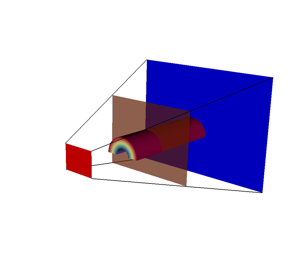
Fig. 8.24 A plot of 5 meshes: the actual mesh that the query used to generate results, the 3 imaging planes, and the ray corners mesh.

The ray corners mesh is useful because no matter the chosen dimensions of the output image, the ray corners mesh always will only contain 4 lines. Therefore it is cheap to render in a tool like VisIt, and it gives a general sense of what is going on. But for those who wish to see all of the rays used in the ray trace, the following will be useful.

The second rays mesh provided is the ray mesh, which provides all the rays used in the ray trace, represented as lines in Blueprint. A note of caution: depending on how many rays are used in the ray trace, this mesh could be expensive to render, hence the inclusion of the ray corners mesh.

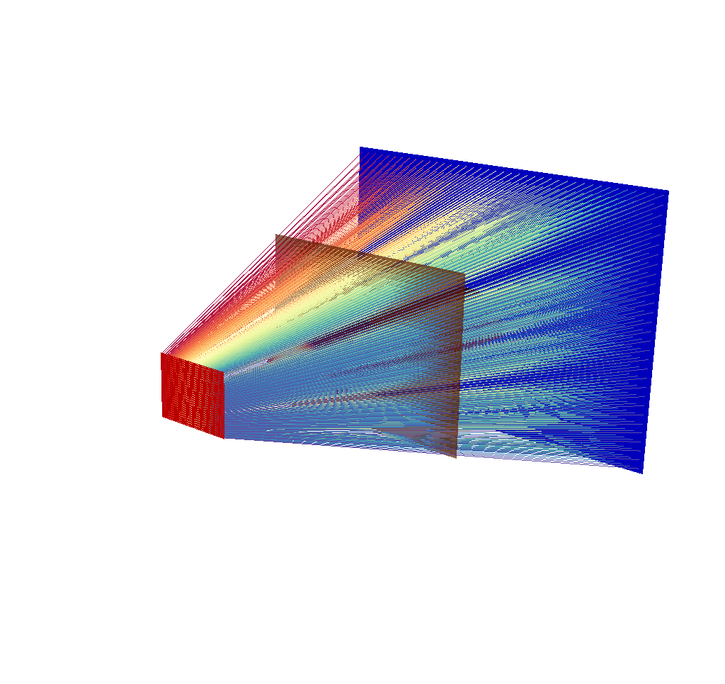
Fig. 8.25 There are 40x30 rays in this image, corresponding to an x ray image output of 40x30 pixels.

Depending on the chosen dimensions of the output image, this mesh can contain thousands of lines. See the following image, which is the same query as the previous image, but this time with 400x300 pixels.

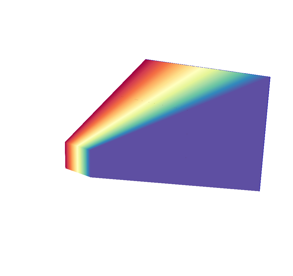
Fig. 8.26 There are 400x300 rays in this image, corresponding to an x ray image output of 400x300 pixels.

This render is far less useful. Even the imaging planes have been swallowed up, and the input mesh is completely hidden. There are a couple quick solutions to this problem. The first solution is to temporarily run the query with less rays (i.e. lower the image dimensions) until the desired understanding of what the simulated x ray detector is looking at has been achieved, then switch back to the large number of pixels/rays. This can be done quickly, as the ray trace is the performance bottleneck for the x ray image query. Here are examples:

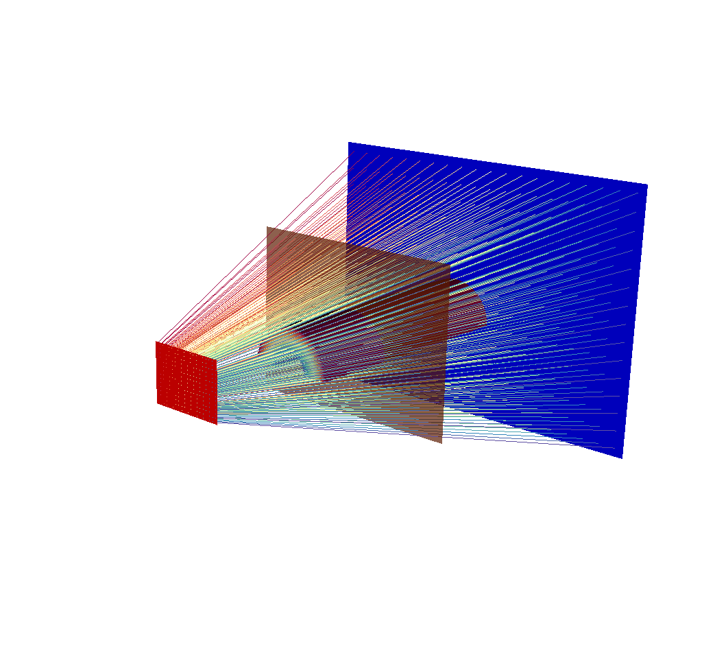
Fig. 8.27 There are 20x15 rays in this image, corresponding to an x ray image output of 20x15 pixels.

Fig. 8.28 There are 8x6 rays in this image, corresponding to an x ray image output of 8x6 pixels.

These renders are less overwhelming, they can be generated quickly, and they get across a good amount of information. But there is another option that does not require losing information.

The second solution is adjusting the opacity of the rays using VisIt. Here is a view of a different run of the query, this time with the simulated x ray detector to the side of the input mesh.

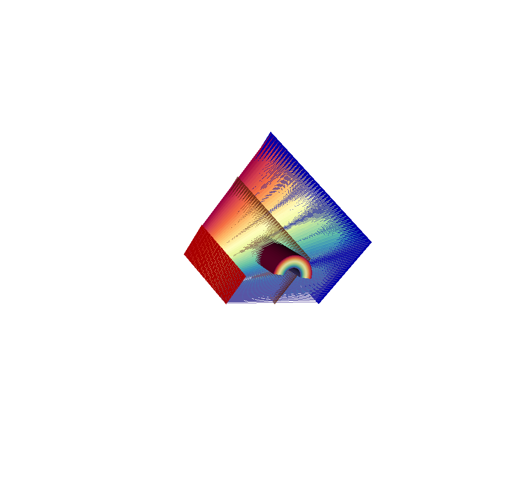
Fig. 8.29 There are 40x30 rays in this image, corresponding to an x ray image output of 40x30 pixels. This is a view of a different run of the query from the images shown thus far.

Even with only 40x30 rays, it is already hard to see the input mesh underneath the rays. With VisIt, it is very easy to adjust the opacity of the rays and make them semitransparent. Here is the same view but with the opacity adjusted for greater visibility.

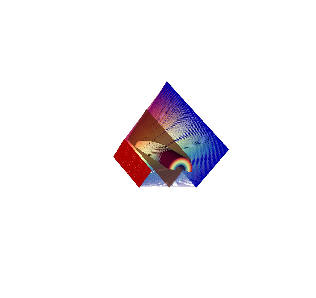
Fig. 8.30 The 40x30 rays have had their opacity lowered for greater visibility.

Here is the same view but with 400x300 rays.

Fig. 8.31 There are 400x300 rays in this image, corresponding to an x ray image output of 40x30 pixels. The rays totally obscure the geometry.

And here is the same view with 400x300 rays but with the ray opacity lowered.

Fig. 8.32 The 400x300 rays have had their opacity lowered for greater visibility.

Hopefully it is clear at this point that there are multiple ways of looking at the rays that are used in the ray trace.

To extract this mesh data with Python, see Accessing Everything Else. To visualize these meshes with VisIt, see Visualizing the Rays Meshes. Now we will take a look at another example inspired by the example in Overview of Output, but this time with only the rays meshes fully realized:

state:
  time: 4.8
  cycle: 48
  xray_view:
    ...
  xray_query:
    ...
  xray_data:
    ...
  domain_id: 0
coordsets:
  image_coords:
    ...
  spatial_coords:
    ...
  spatial_energy_reduced_coords:
    ...
  spectra_coords:
    ...
  near_plane_coords:
    ...
  view_plane_coords:
    ...
  far_plane_coords:
    ...
  ray_corners_coords:
    type: "explicit"
    values:
      x: [-11.1966131618919, 24.5299468925895, 11.1966131618919, ..., -11.1966131618919, 24.5299468925895]
      y: [10.8974596211551, -15.8974596211551, 10.8974596211551, ..., -5.89745962115514, 20.8974596211551]
      z: [-40.0, 60.0, -40.0, ..., -40.0, 60.0]
  ray_coords:
    type: "explicit"
    values:
      x: [11.1686216289872, 11.1686216289872, 11.1686216289872, ..., 24.4686220253581, 24.4686220253581]
      y: [10.8694680890846, 10.8134850249436, 10.7575019608025, ..., 20.7134850249436, 20.8361347557513]
      z: [-40.0, -40.0, -40.0, ..., 60.0, 60.0]
topologies:
  image_topo:
    ...
  spatial_topo:
    ...
  spatial_energy_reduced_topo:
    ...
  spectra_topo:
    ...
  near_plane_topo:
    ...
  view_plane_topo:
    ...
  far_plane_topo:
    ...
  ray_corners_topo:
    type: "unstructured"
    coordset: "ray_corners_coords"
    elements:
      shape: "line"
      connectivity: [0, 1, 2, ..., 6, 7]
  ray_topo:
    type: "unstructured"
    coordset: "ray_coords"
    elements:
      shape: "line"
      connectivity: [0, 120000, 1, ..., 119999, 239999]
fields:
  intensities:
    ...
  path_length:
    ...
  intensities_spatial:
    ...
  path_length_spatial:
    ...
  intensities_spatial_energy_reduced:
    ...
  path_length_spatial_energy_reduced:
    ...
  intensities_spectra:
    ...
  path_length_spectra:
    ...
  near_plane_field:
    ...
  view_plane_field:
    ...
  far_plane_field:
    ...
  ray_corners_field:
    topology: "ray_corners_topo"
    association: "element"
    volume_dependent: "false"
    values: [0.0, 0.0, 0.0, 0.0]
  ray_field:
    topology: "ray_topo"
    association: "element"
    volume_dependent: "false"
    values: [0.0, 1.0, 2.0, ..., 119998.0, 119999.0]

The Blueprint mesh setup may be familiar by now after reading the other sections, particularly the Basic Mesh Output section, so we will only mention here that for each ray mesh, there are the usual three components, a coordinate set, a topology, and a field. The topology tells Blueprint that the shapes in question are lines, which is how we represent the rays.

The final topic of note in this section ties in to the following questions: Why are the rays all different colors? What do the colors mean? The answer is that the colors mean nothing, and the color choices are entirely arbitrary. These colors come from the field values under fields/ray_field, which run from 0 to n, where n is the number of rays. We found that if all the rays were the same color, the resulting render was much harder to visually parse. Of course, rendering the rays as one color is still an option. With VisIt, one need only draw a Mesh Plot of the mesh_ray_topo as opposed to a Pseudocolor Plot of the mesh_ray_topo/ray_field.

To extract this mesh data with Python, see Accessing Everything Else. To visualize these meshes with VisIt, see Visualizing the Rays Meshes.

8.3.4.2.4. Spatial Extents Meshes

The spatial extents mesh and the spatial energy reduced mesh are two additional pieces that we include with the Conduit Output.

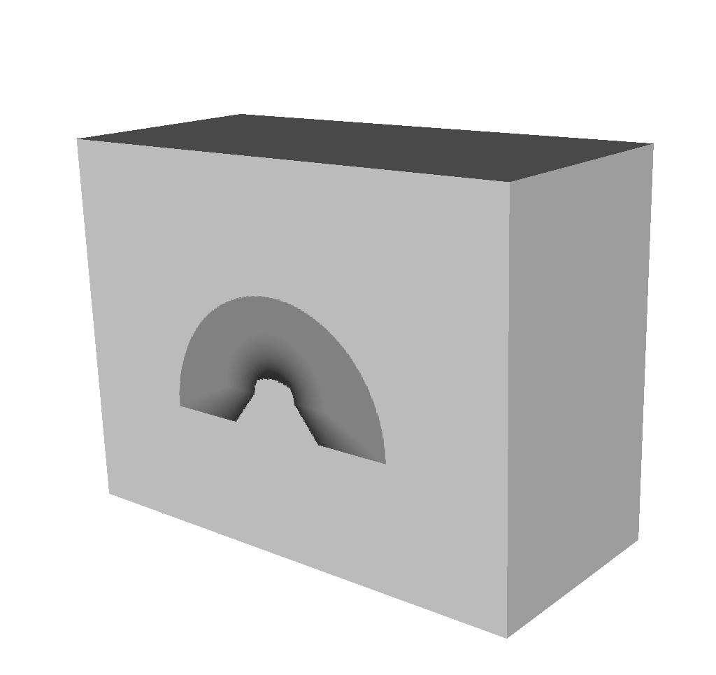
Fig. 8.33 The Spatial Extents Mesh visualized using VisIt.

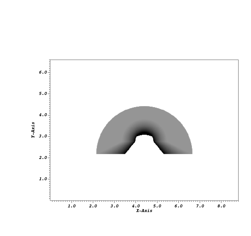
Fig. 8.34 The Spatial Energy Reduced Mesh visualized using VisIt.

The first of these two is the Spatial Extents Mesh, which bears great similarity to that of the Basic Mesh Output. The Basic Mesh Output gives users a picture, in a sense, that was taken by the simulated x ray detector. That picture lives in image space, where the x and y dimensions are given in pixels, and the z dimension represents the number of energy group bins.

The spatial extents mesh is the same picture that was taken by the simulated x ray detector, but living in physical space. Instead of the x and y dimensions representing pixels, the x and y dimensions here represent spatial values. In the example below, these dimensions are in centimeters. The x and y values run from 0 to the detector width and height values, respectively, that appear in the Other Metadata section of the Blueprint output. The z dimension represents actual energy group bins. These are values that were passed in via the query arguments (see Standard Arguments for more information). In the Blueprint example below, the z dimension represents Kiloelectron Volts.

Another way to think about the spatial extents mesh is if the basic mesh output was resized and then pasted on top of the near plane mesh (Imaging Planes), you would get the spatial extents mesh (ignoring the z dimension). The rationale for including this mesh is twofold:

1. It provides yet another view of the data. Perhaps seeing the output with spatial coordinates in x and y is more useful than seeing it with pixel coordinates. If parallel projection is used (Complete Camera Specification), the spatial view of the output is far more useful.

2. This mesh acts as a container for various interesting pieces of data that users may want to pass through the query. This is the destination for the spatial_units and energy_units (Units), which show up under coordsets/spatial_coords/units. This is also where the energy group bounds (Standard Arguments) appear in the output, under coordsets/spatial_coords/values/z.

If the energy group bounds were not provided by the user, or the provided bounds do not match the actual number of bins used in the ray trace, then there will be a message explaining what went wrong under coordsets/spatial_coords/info, and the z values will go from 0 to n where n is the number of bins.

The other mesh that is included, the Spatial Energy Reduced Mesh, is a simplification of the Spatial Extents Mesh. We collapse the information in the Spatial Extents Mesh into 2D by taking, for each x and y element (or pixel), the field value (either intensities or path lengths) to be the sum of the field values along the z axis scaled by the corresponding energy bin widths, if they are provided by the user.

To extract this mesh data with Python, see Accessing the Spatial Extents Meshes Data. To visualize these meshes with VisIt, see Visualizing the Spatial Extents Meshes. The following is the example from Overview of Output, but with only the spatial extents meshes fully realized:

state:
  time: 4.8
  cycle: 48
  xray_view:
    ...
  xray_query:
    ...
  xray_data:
    ...
  domain_id: 0
coordsets:
  image_coords:
    ...
  spatial_coords:
    type: "rectilinear"
    values:
      x: [-0.0, -0.0559830658094596, -0.111966131618919, ..., -22.3372432579744, -22.3932263237838]
      y: [-0.0, -0.0559830641410342, -0.111966128282068, ..., -16.7389361781692, -16.7949192423103]
      z: [3.7, 4.2]
    units:
      x: "cm"
      y: "cm"
      z: "kev"
    labels:
      x: "width"
      y: "height"
      z: "energy_group"
  spatial_energy_reduced_coords:
    type: "rectilinear"
    values:
      x: [-0.0, -0.0559830658094596, -0.111966131618919, ..., -22.3372432579744, -22.3932263237838]
      y: [-0.0, -0.0559830641410342, -0.111966128282068, ..., -16.7389361781692, -16.7949192423103]
    units:
      x: "cm"
      y: "cm"
    labels:
      x: "width"
      y: "height"
  spectra_coords:
    ...
  near_plane_coords:
    ...
  view_plane_coords:
    ...
  far_plane_coords:
    ...
  ray_corners_coords:
    ...
  ray_coords:
    ...
topologies:
  image_topo:
    ...
  spatial_topo:
    coordset: "spatial_coords"
    type: "rectilinear"
  spatial_energy_reduced_topo:
    coordset: "spatial_energy_reduced_coords"
    type: "rectilinear"
  spectra_topo:
    ...
  near_plane_topo:
    ...
  view_plane_topo:
    ...
  far_plane_topo:
    ...
  ray_corners_topo:
    ...
  ray_topo:
    ...
fields:
  intensities:
    ...
  path_length:
    ...
  intensities_spatial:
    topology: "spatial_topo"
    association: "element"
    units: "intensity units"
    values: [0.281004697084427, 0.281836241483688, 0.282898783683777, ..., 0.0, 0.0]
    strides: [1, 400, 120000]
  path_length_spatial:
    topology: "spatial_topo"
    association: "element"
    units: "path length metadata"
    values: [2.46405696868896, 2.45119333267212, 2.43822622299194, ..., 0.0, 0.0]
    strides: [1, 400, 120000]
  intensities_spatial_energy_reduced:
    topology: "spatial_energy_reduced_topo"
    association: "element"
    values: [0.70251174271, 0.7045906037, 0.7072469592, ..., 0.0, 0.0]
  path_length_spatial_energy_reduced:
    topology: "spatial_energy_reduced_topo"
    association: "element"
    values: [6.16014242172, 6.12798333168, 6.09556555748, ..., 0.0, 0.0]
  intensities_spectra:
    ...
  path_length_spectra:
    ...
  near_plane_field:
    ...
  view_plane_field:
    ...
  far_plane_field:
    ...
  ray_corners_field:
    ...
  ray_field:
    ...

As can be seen from the example, this view of the output is very similar to the Basic Mesh Output. It has all the same components, a coordinate set spatial_coords, a topology spatial_topo, and fields intensities_spatial and path_length_spatial. The topology and fields are exact duplicates of those found in the Basic Mesh Output. The Spatial Energy Reduced Mesh is similar, but notable in the sense that it is missing the z dimension.

The impetus for including the spatial extents mesh was originally to include spatial coordinates as part of the metadata, but later on it was decided that the spatial coordinates should be promoted to be a proper Blueprint coordset. We then duplicated the existing topology and fields from the Basic Mesh Output so that the spatial extents coordset could be part of a valid Blueprint mesh, and could thus be visualized using VisIt.

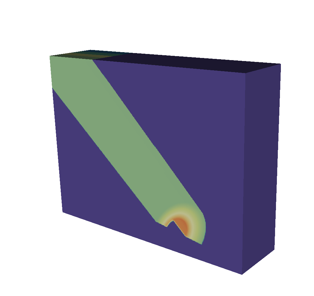
Fig. 8.35 The spatial extents mesh looks very similar to the basic mesh output. It is in 3D and the z dimension represents the energy group bounds, which in this example run from 0 to 12.

To extract this mesh data with Python, see Accessing the Spatial Extents Meshes Data. To visualize these meshes with VisIt, see Visualizing the Spatial Extents Meshes.

8.3.4.2.5. 1D Spectra Curves

To provide yet another view of the intensities and path lengths data, we include two curves, represented as blueprint meshes.

Fig. 8.36 One of the 1D Spectra Curves visualized using VisIt.

Similar to the Spatial Energy Reduced Mesh (Spatial Extents Meshes), the provided mesh is a dimension collapse of the Spatial Extents Mesh. However, instead of collapsing the z dimension (energy group bounds) by taking a sum, we collapse the x and y dimensions (spatial extents). Thus we are left with a 1D curve, where for each energy group bin, there is one field value that is the result of summing the fields values (intensities or path lengths scaled by the spatial extents of each pixel) for each z-plane. There is one curve for the intensities and one curve for the path lengths.

To extract this mesh data with Python, see Accessing the 1D Spectra Curves Data. To visualize this mesh with VisIt, see Visualizing the 1D Spectra Curves. The following is the example from Overview of Output, but with the Blueprint mesh representing the 1D Spectra Curves fully realized:

state:
  time: 4.8
  cycle: 48
  xray_view:
    ...
  xray_query:
    ...
  xray_data:
    ...
  domain_id: 0
coordsets:
  image_coords:
    ...
  spatial_coords:
    ...
  spatial_energy_reduced_coords:
    ...
  spectra_coords:
    type: "rectilinear"
    values:
      x: [0.0, 1.0, 2.0, 3.0, 4.0]
    units:
      x: "kev"
    labels:
      x: "energy_group"
  near_plane_coords:
    ...
  view_plane_coords:
    ...
  far_plane_coords:
    ...
  ray_corners_coords:
    ...
  ray_coords:
    ...
topologies:
  image_topo:
    ...
  spatial_topo:
    ...
  spatial_energy_reduced_topo:
    ...
  spectra_topo:
    coordset: "spectra_coords"
    type: "rectilinear"
  near_plane_topo:
    ...
  view_plane_topo:
    ...
  far_plane_topo:
    ...
  ray_corners_topo:
    ...
  ray_topo:
    ...
fields:
  intensities:
    ...
  path_length:
    ...
  intensities_spatial:
    ...
  path_length_spatial:
    ...
  intensities_spatial_energy_reduced:
    ...
  path_length_spatial_energy_reduced:
    ...
  intensities_spectra:
    topology: "spectra_topo"
    association: "element"
    values: [1.64416097681804, 3.31540252150611, 6.65558651188286, 4.98593527287638]
  path_length_spectra:
    topology: "spectra_topo"
    association: "element"
    values: [356.40441526888, 712.808830537761, 1425.61766107552, 1069.21324547146]
  near_plane_field:
    ...
  view_plane_field:
    ...
  far_plane_field:
    ...
  ray_corners_field:
    ...
  ray_field:
    ...

Again, we have the typical 3 components of a Blueprint mesh. This is no different than the other Blueprint meshes, despite the fact that this will be represented differently under the hood in VisIt to make it appear as a curve when plotted.

To extract this mesh data with Python, see Accessing the 1D Spectra Curves Data. To visualize this mesh with VisIt, see Visualizing the 1D Spectra Curves.

8.3.4.3. Quick Results

One of the advantages of using Conduit Output is the ability to view quick results that give an overview of the output data. In this section, we will briefly discuss three of those quick results. Each of these have been discussed individually in other sections but not all together.

First is the Spatial Energy Reduced Mesh (discussed in greater detail here: Spatial Extents Meshes). This mesh is a 2-dimensional representation of the intensities and path lengths. We have collapsed the energy group bins to arrive at this result. The point of including this is to give a broad, at-a-glance view of the data. If, for example, many energy group bins contain uninteresting data, but a few have important structure, it can be difficult to get at that information using the Basic Mesh Output or the 3-dimensional Spatial Extents Mesh. Because the Spatial Energy Reduced Mesh fields are the result of taking the sum of the intensities and path lengths fields across all the energy group bins, that structure will be visible at a glance in a render of this mesh, as opposed to needing to be hunted for using VisIt’s slicing and threshold tools, for example.

Fig. 8.37 A render of the spatial energy reduced mesh intensities, viewing our typical half cylinder example from the side.

To render this, see Visualizing the Spatial Extents Meshes.

Next up are the Spectra Curves (discussed in greater detail here: 1D Spectra Curves). This mesh is a 1-dimensional representation of the intensities and path lengths. Instead of collapsing the energy group bins, we have collapsed the x and y spatial dimensions to arrive at this result. Thus we get a curve that associates energy levels with intensities or path lengths. It may be helpful to view this curve with a logarithmic scale. Now it is possible to see exactly how intensities or path length data varies across energy levels.

Fig. 8.38 A render of the intensities spectra curve. The X dimension represents energy and the Y dimension represents intensities.

To render this, see Visualizing the 1D Spectra Curves.

The final quick view of the data that we will cover in this section are the intensities and path lengths maximums and minimums included as part of the Metadata. For context, we have opted to calculate the maximum and minimum intensity and path length values and output that information under Other Metadata. These four values are not necessarily a “view” of the data, but they do give a shallow sense of what to expect. If all four are zero, for example, that means that all output images are blank. See Troubleshooting for more information about that case. Otherwise, these four values can yield a quick sanity check, as hopefully maximum and minimum intensity and path length values are within reason. See Accessing the Metadata for information on extracting these values from the Metadata.

8.3.4.4. Pitfalls

Despite all of these features being added to the X Ray Image Query to facilitate usability, there are still cases where confusion can arise. One such case is where the spatial extents mesh can appear to be upside down. Consider the following:

Fig. 8.39 An input mesh, imaging planes, and ray corners, viewed from the side.

If we adjust the query so that the near plane is further away (say maybe from -15 to -35), we will see this:

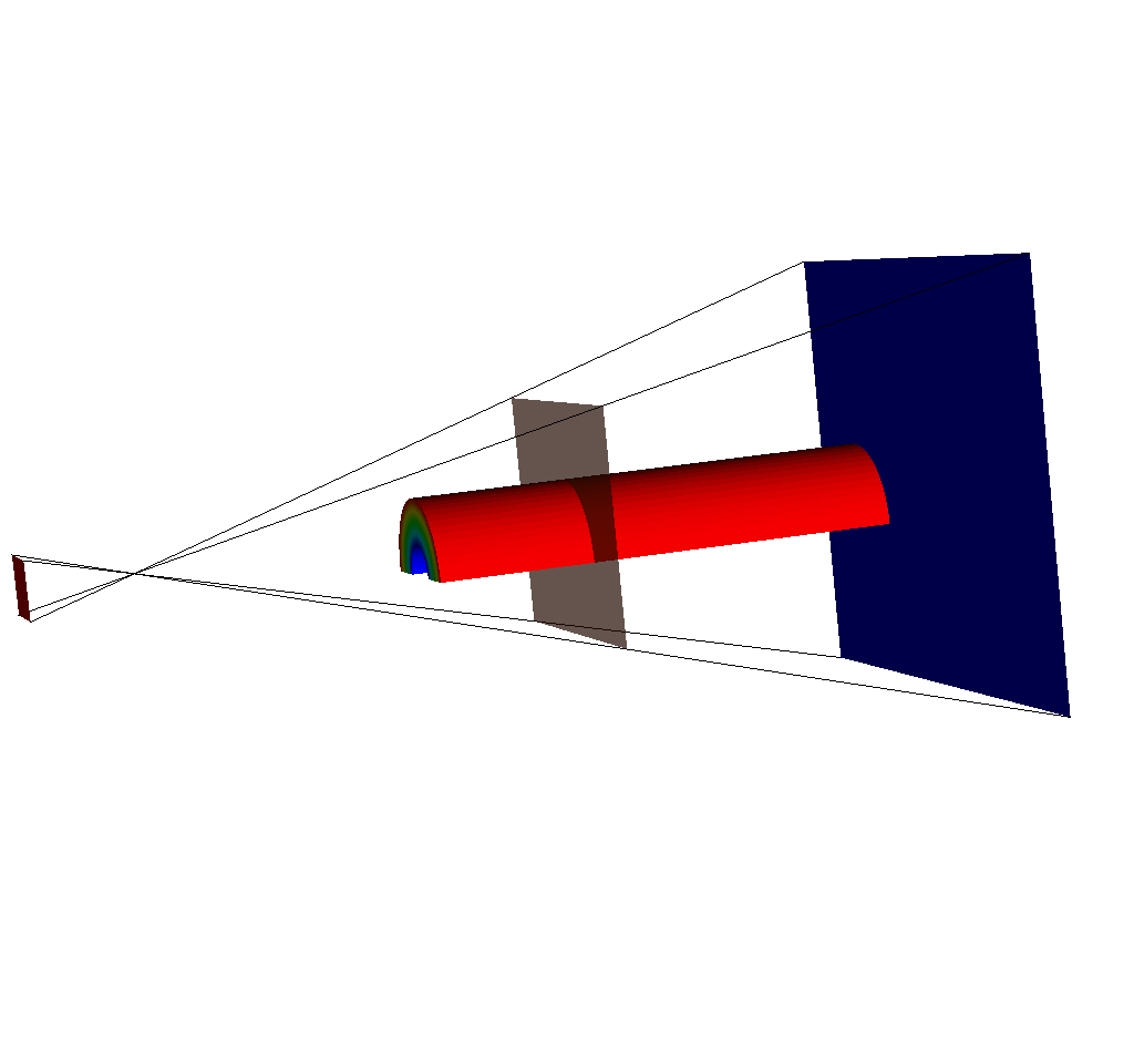
Fig. 8.40 The same set of plots as before, except this time the near plane has been moved back.

Fig. 8.41 Another view of this situation.

The near plane has passed out of the view frustum. This is because the view frustum is determined by the view_angle argument (see Complete Camera Specification). In this case, the query is using the default value of 30 degrees, and because the near plane is far enough back, it is outside the frustum.

So what does this mean for the other query results? It means that while we’d expect our Spatial Extents Mesh (Spatial Extents Meshes) to look like this:

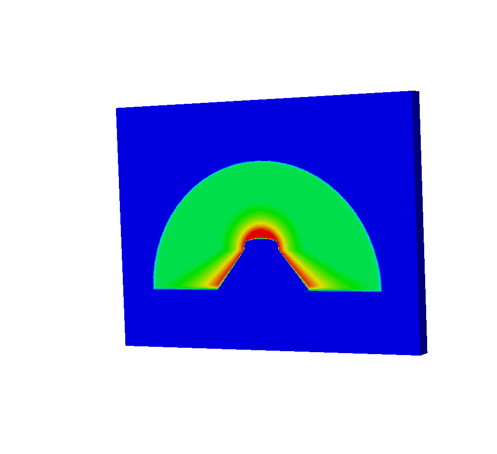
Fig. 8.42 The spatial extents mesh as we’d expect to see from running the query.

It will actually look like this:

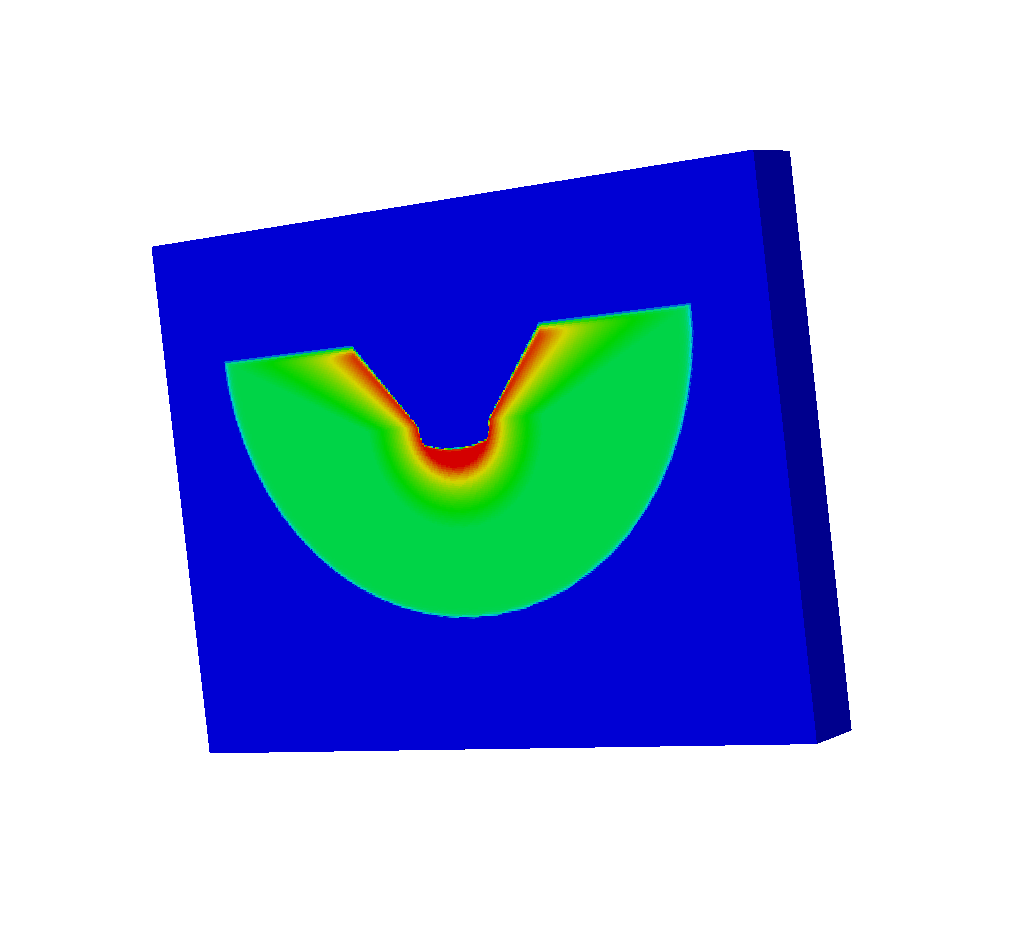
Fig. 8.43 The upside-down spatial extents mesh that we actually get from running the query.

Why is the mesh upside-down? The spatial extents mesh is upside-down because the simulated x ray detector is upside down. Previously, in the Spatial Extents Meshes section we described the spatial extents mesh as though we had taken the Basic Mesh Output, resized it, and pasted it on top of the near plane. That is exactly what is happening here. The spatial extents mesh is upside down because the near plane is upside down.

Here are the same images as above, but this time, in each one, the upper right corner of each imaging plane is marked in green:

Fig. 8.44 An input mesh, imaging planes, and ray corners, viewed from the side. Note the upper right corner of each imaging plane is marked in green.

If we adjust the query so that the near plane is further away (say maybe from -15 to -35), we will see this:

Fig. 8.45 The same set of plots as before, except this time the near plane has been moved back. Note the upper right corner of each imaging plane is marked in green. For the near plane (red), the upper right corner is not where we would expect.

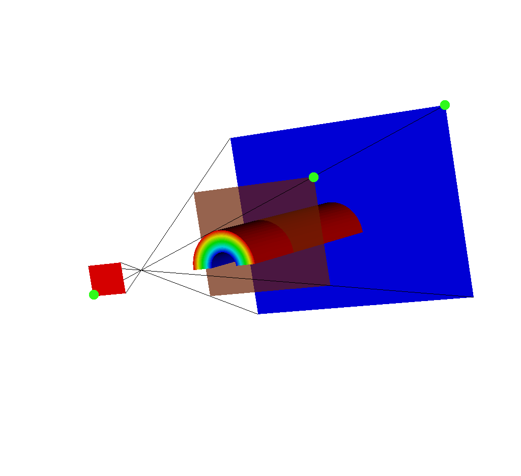
Fig. 8.46 Another view of this situation. Note the upper right corner of each imaging plane is marked in green. The upper right corner for the near plane (red) is on the bottom left because the near plane is reflected across the x and y axes.

Following the ray corners, we see that the upper right corner for the near plane is actually on the bottom left, because the whole near plane has been reflected to accommodate the fact that it is behind the frustum. This explains why the spatial extents mesh appears upside down; it is actually reflected across the x and y axes.

This special case will trigger a warning message if VisIt is run with -debug 1.

8.3.4.5. Visualizing with VisIt

One of the advantages of using one of the Conduit Output types is that it is easy to both look at the raw data and generate x ray images. This section will cover generating x ray images using VisIt as well as visualizing the other components of the Conduit Output.

The later Python code examples assume that the following has already been run:

# The file containing the mesh I wish to ray trace
OpenDatabase("testdata/silo_hdf5_test_data/curv3d.silo")

# The query requires a plot to be visible
AddPlot("Pseudocolor", "d")
DrawPlots()

# Call the query
params = dict()
params["image_size"] = (400, 300)
# One of the Blueprint output types
params["output_type"] = "hdf5"
params["focus"] = (0., 2.5, 10.)
params["perspective"] = 1
params["near_plane"] = -25.
params["far_plane"] = 25.
params["vars"] = ("d", "p")
# Dummy values to demonstrate functionality
params["energy_group_bounds"] = [2.7, 6.2]
params["parallel_scale"] = 10.
Query("XRay Image", params)

# Open the file that was output from the query.
# In this case it is called "output.root"
OpenDatabase("output.root")

Once the query has been run, to visualize each constituent part of the output, follow these steps in Python:

8.3.4.5.1. Visualizing the Basic Mesh Output

First we will cover visualizing the Basic Mesh Output.

# Make sure we have a clean slate for ensuing visualizations.
DeleteAllPlots()

# Add a pseudocolor plot of the intensities
AddPlot("Pseudocolor", "mesh_image_topo/intensities")

# Alternatively add a plot of the path length instead
# AddPlot("Pseudocolor", "mesh_image_topo/path_length")

DrawPlots()

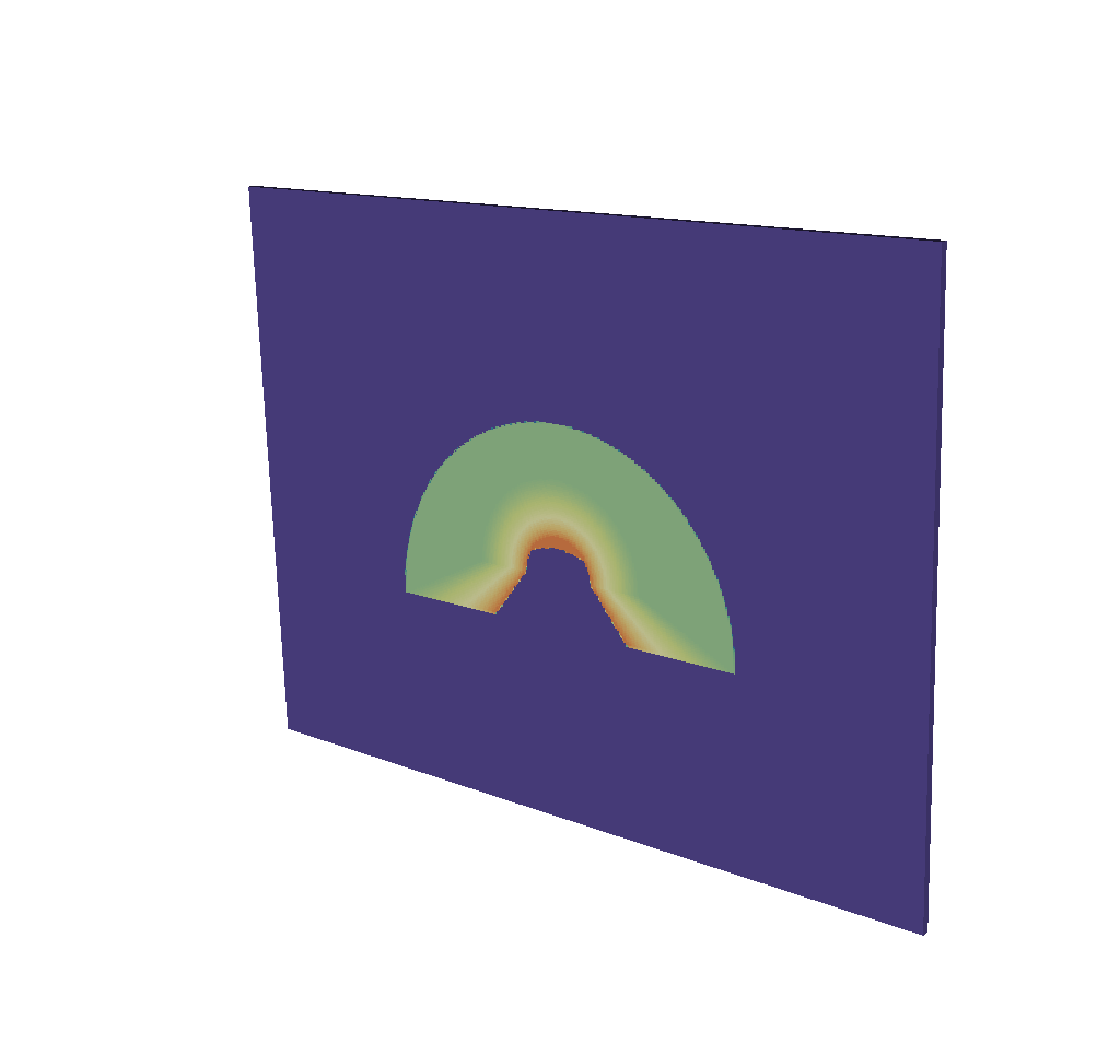
Fig. 8.47 A visualization of the basic mesh output.

To make the output look like an x ray image, it is simple to change the color table.

# Make sure the plot you want to change the color of is active
PseudocolorAtts = PseudocolorAttributes()
PseudocolorAtts.colorTableName = "xray"
SetPlotOptions(PseudocolorAtts)

Fig. 8.48 A visualization of the basic mesh output using the x ray color table.

8.3.4.5.2. Visualizing the Imaging Planes

To simply render the Imaging Planes on top of your simulation data we will do the following:

# Make sure we have a clean slate for ensuing visualizations.
DeleteAllPlots()

# First we wish to make sure that the input mesh is visible
ActivateDatabase("testdata/silo_hdf5_test_data/curv3d.silo")
AddPlot("Pseudocolor", "d")
DrawPlots()

# Then we want to go back to the output file and visualize the imaging planes
ActivateDatabase("output.root")
AddPlot("Pseudocolor", "mesh_near_plane_topo/near_plane_field")
AddPlot("Pseudocolor", "mesh_view_plane_topo/view_plane_field")
AddPlot("Pseudocolor", "mesh_far_plane_topo/far_plane_field")
DrawPlots()

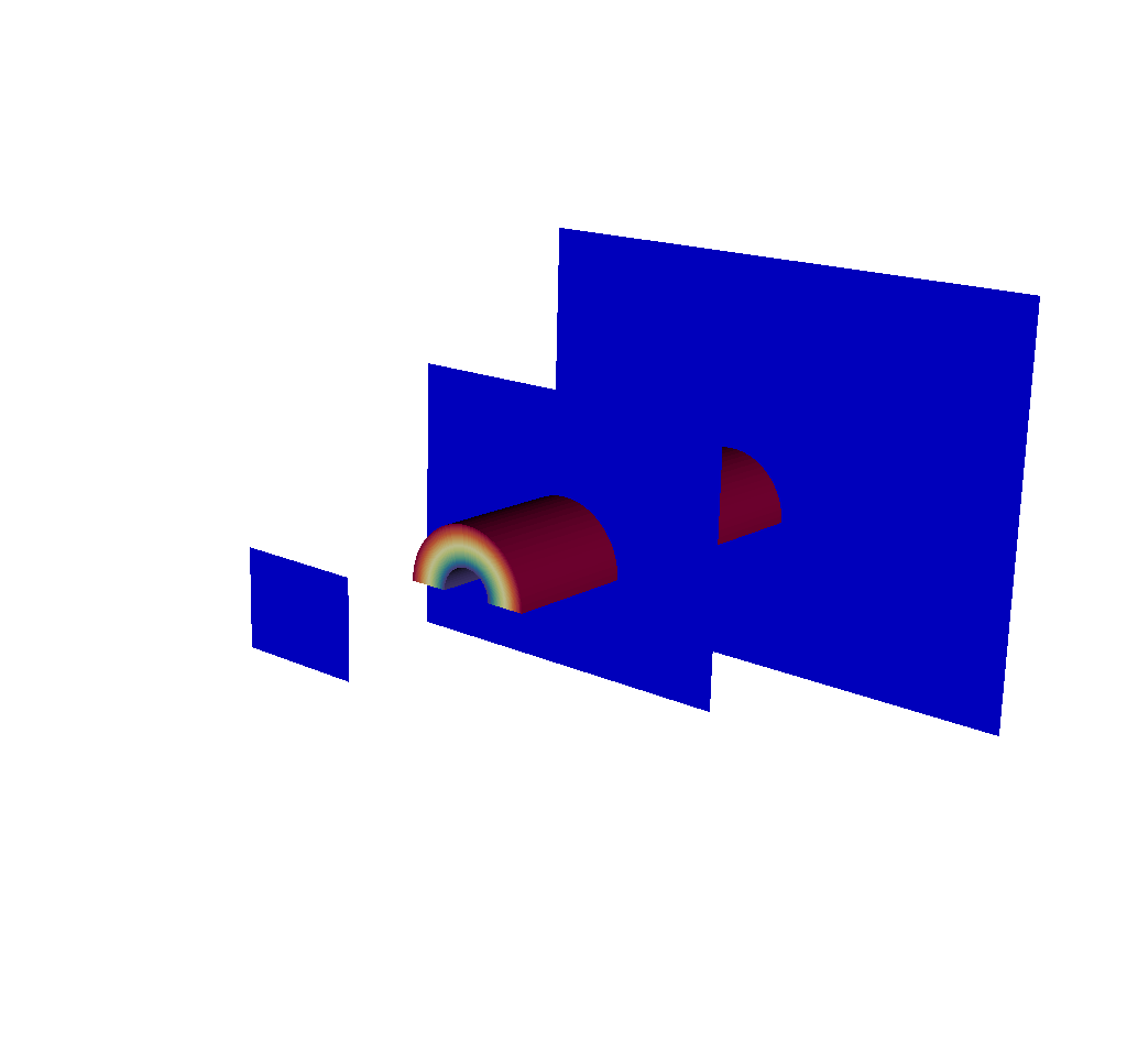
Fig. 8.49 A visualization of the input mesh along with the imaging planes.

This will color the imaging planes all the same color. To make them distinct colors like in all the examples throughout this documentation, we can do the following:

# Make the plot of the near plane active
SetActivePlots(1)
PseudocolorAtts = PseudocolorAttributes()
# We invert the color table so that it is a different color from the far plane
PseudocolorAtts.invertColorTable = 1
SetPlotOptions(PseudocolorAtts)

# Make the plot of the view plane active
SetActivePlots(2)
PseudocolorAtts = PseudocolorAttributes()
PseudocolorAtts.colorTableName = "Oranges"
PseudocolorAtts.invertColorTable = 1
PseudocolorAtts.opacityType = PseudocolorAtts.Constant  # ColorTable, FullyOpaque, Constant, Ramp, VariableRange
# We lower the opacity so that the view plane does not obstruct our view of anything.
PseudocolorAtts.opacity = 0.7
SetPlotOptions(PseudocolorAtts)

# leave the far plane as is

Fig. 8.50 A visualization of the input mesh along with the imaging planes, where they have had their colors adjusted.

8.3.4.5.3. Visualizing the Rays Meshes

For the sake of visual clarity, as we visualize the Rays Meshes, we will build on the imaging planes visualization from above. To visualize the ray corners, it is a simple matter of doing the following:

# This plots the ray corners mesh
AddPlot("Mesh", "mesh_ray_corners_topo")

# Alternatively, we could plot the dummy field that is included, but
# plotting just the mesh will make sure the plot is in black, which
# looks better with the colors we are using to paint the imaging planes.
# AddPlot("Pseudocolor", "mesh_ray_corners_topo/ray_corners_field")

DrawPlots()

# The next few lines of code make the rays appear thicker for visual clarity.
MeshAtts = MeshAttributes()
MeshAtts.lineWidth = 1
SetPlotOptions(MeshAtts)

Fig. 8.51 A visualization of the input mesh, the imaging planes, and the ray corners.

Now we will visualize all of the rays.

AddPlot("Pseudocolor", "mesh_ray_topo/ray_field")
DrawPlots()

Fig. 8.52 A visualization of the input mesh, the imaging planes, the ray corners, and the rays.

As discussed in the Rays Meshes section, this picture is not very helpful, so we will reduce the opacity for greater visual clarity:

PseudocolorAtts = PseudocolorAttributes()
PseudocolorAtts.opacityType = PseudocolorAtts.Constant  # ColorTable, FullyOpaque, Constant, Ramp, VariableRange
PseudocolorAtts.opacity = 0.5
SetPlotOptions(PseudocolorAtts)

Fig. 8.53 A visualization of the input mesh, the imaging planes, the ray corners, and the rays, with their opacity adjusted.

See the Rays Meshes section for more tips for making sense of the rays.

8.3.4.5.4. Visualizing the Spatial Extents Meshes

Visualizing the Spatial Extents Meshes should be very similar to Visualizing the Basic Mesh Output.

First we render the spatial extents mesh:

# Make sure we have a clean slate for ensuing visualizations.
DeleteAllPlots()

# Add a pseudocolor plot of the intensities
AddPlot("Pseudocolor", "mesh_spatial_topo/intensities_spatial")

# Alternatively add a plot of the path length instead
# AddPlot("Pseudocolor", "mesh_spatial_topo/path_length_spatial")

DrawPlots()

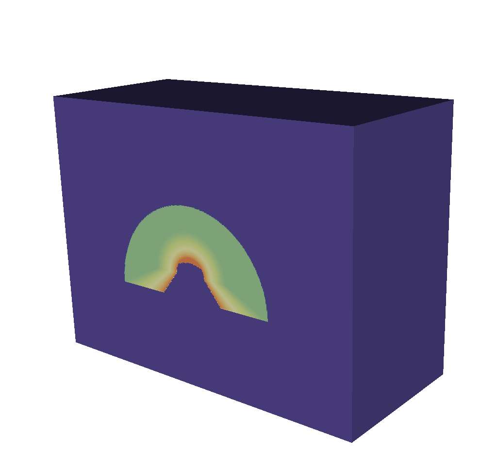
Fig. 8.54 A visualization of the spatial extents mesh.

To make the output look like an x ray image, it is simple to change the color table.

# Make sure the plot you want to change the color of is active
PseudocolorAtts = PseudocolorAttributes()
PseudocolorAtts.colorTableName = "xray"
SetPlotOptions(PseudocolorAtts)

Fig. 8.55 A visualization of the spatial extents mesh using the x ray color table.

And then we render the spatial energy reduced mesh:

# Make sure we have a clean slate for ensuing visualizations.
DeleteAllPlots()

# Add a pseudocolor plot of the intensities
AddPlot("Pseudocolor", "mesh_spatial_energy_reduced_topo/intensities_spatial_energy_reduced")

# Alternatively add a plot of the path length instead
# AddPlot("Pseudocolor", "mesh_spatial_energy_reduced_topo/intensities_spatial_energy_reduced")

DrawPlots()

# Change to x ray color table

# Make sure the plot you want to change the color of is active
PseudocolorAtts = PseudocolorAttributes()
PseudocolorAtts.colorTableName = "xray"
SetPlotOptions(PseudocolorAtts)

Fig. 8.56 A visualization of the spatial energy reduced mesh using the x ray color table.

8.3.4.5.5. Visualizing the 1D Spectra Curves

Visualizing the 1D Spectra Curves is slightly different than visualizing the other Blueprint meshes. Because the Blueprint mesh is 1-dimensional, VisIt will interpret it as a curve. So, instead of adding a Pseudocolor plot, we will add a Curve plot instead.

# Make sure we have a clean slate for ensuing visualizations.
DeleteAllPlots()

# Add a curve plot of the intensities
AddPlot("Curve", "mesh_spectra_topo/intensities_spectra")

# Alternatively add a plot of the path length instead
# AddPlot("Curve", "mesh_spectra_topo/path_length_spectra")

DrawPlots()

# Remove the labels to clean up the image
SetActivePlots(0)
CurveAtts = CurveAttributes()
CurveAtts.showLabels = 0
SetPlotOptions(CurveAtts)

Fig. 8.57 A visualization of the 1D Spectra Curve mesh.

8.3.4.6. Introspecting with Python

We have covered visualizing every component of the Conduit Output in the Visualizing with VisIt section; now we will demonstrate how to access the raw data using Python.

8.3.4.6.1. Getting a General Overview of the Output

See Overview of Output for a visual of what the resulting Conduit tree looks like. First, we will get everything set up.

# make sure we import conduit
import conduit

# this node will be the destination for our output
xrayout = conduit.Node()

# actually perform the load
conduit.relay.io.blueprint.load_mesh(xrayout, "output.root")

Now we are ready to begin extracting data. To produce a Conduit tree like that of the example in Overview of Output, Conduit provides some simple tools:

# To print a condensed overview of the output
print(xrayout["domain_000000"])

# This is the same as
# print(xrayout["domain_000000"].to_summary_string())

# These will only print subsets of children, and for each child
# only a subset of leaf array values so as to not overwhelm the screen.

# The following will print the entirety of the output...
# including every coordinate and field value,
# so use with caution.
print(xrayout["domain_000000"].to_yaml())

These simple features can be used not just on the root of the Conduit tree, but everywhere. We will see these used repeatedly in ensuing examples.

One other useful tool for interrogating a Conduit tree is the childnames() function. We can use xrayout.childnames() to see the names of all the top-level children as a list. In this case, calling xrayout.childnames() would produce ['state', 'coordsets', 'topologies', 'fields']. We can call childnames() on any of the children of xrayout (xrayout["state"].childnames(), for example) to further investigate the layers of the tree.

Additionally, it is possible to iterate through the children of a Conduit node using this:

for child in xrayout.children():
   print(child.name(), child.node())

In general, children are not always named. For our purposes with the X Ray Image Query, they always will be. A node can behave like a python dictionary or a python list; for the latter, index access is possible.

8.3.4.6.2. Accessing the Basic Mesh Output Data

To get a sense of what the Basic Mesh Output looks like, we can run the following:

print("image_coords")
print(xrayout["domain_000000/coordsets/image_coords"])

print("image_topo")
print(xrayout["domain_000000/topologies/image_topo"])

print("intensities")
print(xrayout["domain_000000/fields/intensities"])
print("path_length")
print(xrayout["domain_000000/fields/path_length"])

This produces…

image_coords

type: "rectilinear"
values:
  x: [0, 1, 2, ..., 399, 400]
  y: [0, 1, 2, ..., 299, 300]
  z: [0, 1]
labels:
  x: "width"
  y: "height"
  z: "energy_group"
units:
  x: "pixels"
  y: "pixels"
  z: "bins"

image_topo

coordset: "image_coords"
type: "rectilinear"

intensities

topology: "image_topo"
association: "element"
units: "intensity units"
values: [0.0, 0.0, 0.0, ..., 0.0, 0.0]
strides: [1, 400, 120000]

path_length

topology: "image_topo"
association: "element"
units: "path length metadata"
values: [0.0, 0.0, 0.0, ..., 0.0, 0.0]
strides: [1, 400, 120000]

Note that the long arrays are condensed for the sake of readability. If we wanted to see the entirety of the arrays, we could run print(myconduitnode.to_yaml()) instead of print(myconduitnode).

To actually extract the Basic Mesh Output data and not just see it, we can run the following:

# Extract the actual x values, label, and units
xvals = xrayout["domain_000000/coordsets/image_coords/values/x"]
xlabel = xrayout["domain_000000/coordsets/image_coords/labels/x"]
xunits = xrayout["domain_000000/coordsets/image_coords/units/x"]
# Extracting the same for y and z is similar

# Extract units and values for the intensity output
intensity_units = xrayout["domain_000000/fields/intensities/units"]
intensity_values = xrayout["domain_000000/fields/intensities/values"]
# Extracting the same for path_length is similar

These variables can be printed, manipulated, iterated over, etc.

8.3.4.6.3. Accessing the Metadata

Again, to get an overview of the Metadata, it is simple to print the state branch:

# get an overview of the metadata
print(xrayout["domain_000000/state"])

# see all the metadata
print(xrayout["domain_000000/state"].to_yaml())

The following code extracts each of the values. First is top level Metadata:

time = xrayout["domain_000000/state/time"]
cycle = xrayout["domain_000000/state/cycle"]

Next up is View Parameters:

normalx = xrayout["domain_000000/state/xray_view/normal/x"]
normaly = xrayout["domain_000000/state/xray_view/normal/y"]
normalz = xrayout["domain_000000/state/xray_view/normal/z"]

focusx = xrayout["domain_000000/state/xray_view/focus/x"]
focusy = xrayout["domain_000000/state/xray_view/focus/y"]
focusz = xrayout["domain_000000/state/xray_view/focus/z"]

view_upx = xrayout["domain_000000/state/xray_view/view_up/x"]
view_upy = xrayout["domain_000000/state/xray_view/view_up/y"]
view_upz = xrayout["domain_000000/state/xray_view/view_up/z"]

view_angle = xrayout["domain_000000/state/xray_view/view_angle"]
parallel_scale = xrayout["domain_000000/state/xray_view/parallel_scale"]
view_width = xrayout["domain_000000/state/xray_view/view_width"]
non_square_pixels = xrayout["domain_000000/state/xray_view/non_square_pixels"]
near_plane = xrayout["domain_000000/state/xray_view/near_plane"]
far_plane = xrayout["domain_000000/state/xray_view/far_plane"]

image_panx = xrayout["domain_000000/state/xray_view/image_pan/x"]
image_pany = xrayout["domain_000000/state/xray_view/image_pan/y"]

image_zoom = xrayout["domain_000000/state/xray_view/image_zoom"]
perspective = xrayout["domain_000000/state/xray_view/perspective"]
perspective_str = xrayout["domain_000000/state/xray_view/perspective_str"]

Then Query Parameters:

divide_emis_by_absorb = xrayout["domain_000000/state/xray_query/divide_emis_by_absorb"]
divide_emis_by_absorb_str = xrayout["domain_000000/state/xray_query/divide_emis_by_absorb_str"]
num_x_pixels = xrayout["domain_000000/state/xray_query/num_x_pixels"]
num_y_pixels = xrayout["domain_000000/state/xray_query/num_y_pixels"]
num_bins = xrayout["domain_000000/state/xray_query/num_bins"]
abs_var_name = xrayout["domain_000000/state/xray_query/abs_var_name"]
emis_var_name = xrayout["domain_000000/state/xray_query/emis_var_name"]
abs_units = xrayout["domain_000000/state/xray_query/abs_units"]
emis_units = xrayout["domain_000000/state/xray_query/emis_units"]

And finally, Other Metadata:

detector_width = xrayout["domain_000000/state/xray_data/detector_width"]
detector_height = xrayout["domain_000000/state/xray_data/detector_height"]
intensity_max = xrayout["domain_000000/state/xray_data/intensity_max"]
intensity_min = xrayout["domain_000000/state/xray_data/intensity_min"]
path_length_max = xrayout["domain_000000/state/xray_data/path_length_max"]
path_length_min = xrayout["domain_000000/state/xray_data/path_length_min"]
image_topo_order_of_domain_variables = xrayout["domain_000000/state/xray_data/image_topo_order_of_domain_variables"]

8.3.4.6.4. Accessing the Spatial Extents Meshes Data

Because the Spatial Extents Meshes share a lot in common with the Basic Mesh Output, we will only cover here how to extract some of the unique values.

# Extract the actual x, y, and z values
spatial_xvals = xrayout["domain_000000/coordsets/spatial_coords/values/x"]
spatial_yvals = xrayout["domain_000000/coordsets/spatial_coords/values/y"]
energy_group_bounds = xrayout["domain_000000/coordsets/spatial_coords/values/z"]

# Extract the x label
spatial_xlabel = xrayout["domain_000000/coordsets/spatial_coords/labels/x"]
# Extracting the same for y and z is similar

# Extract the spatial and energy units
spatial_xunits = xrayout["domain_000000/coordsets/spatial_coords/units/x"]
spatial_yunits = xrayout["domain_000000/coordsets/spatial_coords/units/y"]
energy_units = xrayout["domain_000000/coordsets/spatial_coords/units/z"]

8.3.4.6.5. Accessing the 1D Spectra Curves Data

The 1D Spectra Curves are similar in structure to the other standard Blueprint meshes.

# Extract the energy group bounds
energy_group_bounds = xrayout["domain_000000/coordsets/spectra_coords/values/x"]

# Extract the label
spectra_label = xrayout["domain_000000/coordsets/spectra_coords/labels/x"]

# Extract the units
spatial_xunits = xrayout["domain_000000/coordsets/spectra_coords/units/x"]

# Extract the field values
intensities_spectra_curve_values = xrayout["domain_000000/fields/intensities_spectra/values"]
# Extracting the same for path_length is similar

8.3.4.6.6. Accessing Everything Else

All of the other data stored in the Conduit output can be accessed in the same way. To get a general sense of what is stored in particular branches of the tree, it is a simple matter of running print(myconduitnode) to quickly get an overview.

8.3.4.7. Troubleshooting

Now that we have explored the Conduit Blueprint output in detail, we can use it to troubleshoot unexpected or strange query results.

8.3.4.7.1. Is my image blank?

This question can be answered without even examining the image (or in the case of the Blueprint output, a render of the Basic Mesh Output). It is as simple as checking if the minimum and maximum values for the intensities and path length are zero. See Other Metadata for more information. These values can be pulled out of the Conduit output with ease, using the following:

import conduit
mesh = conduit.Node()

# In this case, "output.root" is the name of the Blueprint file
# that was output from the query.
conduit.relay.io.blueprint.load_mesh(mesh, "output.root")

# We extract the values from the node.
intensity_max = mesh["domain_000000/state/xray_data/intensity_max"]
intensity_min = mesh["domain_000000/state/xray_data/intensity_min"]
path_length_max = mesh["domain_000000/state/xray_data/path_length_max"]
path_length_min = mesh["domain_000000/state/xray_data/path_length_min"]

print("intensity_max = " + str(intensity_max))
print("intensity_min = " + str(intensity_min))
print("path_length_max = " + str(path_length_max))
print("path_length_min = " + str(path_length_min))

Yielding:

intensity_max = 0.49144697189331055
intensity_min = 0.0
path_length_max = 129.8570098876953
path_length_min = 0.0

If the maximums were also equal to zero, then the image would be blank. Hence, it is possible to quickly programmatically check if the image is blank, without any need for taking the time to look at the image. See Introspecting with Python for more information about extracting data from the query output.

8.3.4.7.2. Why is my image blank?

Is the camera facing the right way? Are the near and far clipping planes in good positions?

This line of questioning can be quickly answered by Visualizing the Imaging Planes and Visualizing the Rays Meshes.

# Make sure the mesh used in the query is already rendered.

# In this case, "output.root" is the name of the Blueprint file
# that was output from the query.
OpenDatabase("output.root")

# Add pseudocolor plots of each of the imaging planes.
AddPlot("Pseudocolor", "mesh_far_plane_topo/far_plane_field")
AddPlot("Pseudocolor", "mesh_view_plane_topo/view_plane_field")
AddPlot("Pseudocolor", "mesh_near_plane_topo/near_plane_field")

# Add a mesh plot of the ray corners.
AddPlot("Mesh", "mesh_ray_corners_topo")

DrawPlots()

Running this code using VisIt should result in renders like those shown in Imaging Planes and Rays Meshes. To make the planes different colors, use VisIt’s color table controls, or see Visualizing the Imaging Planes.

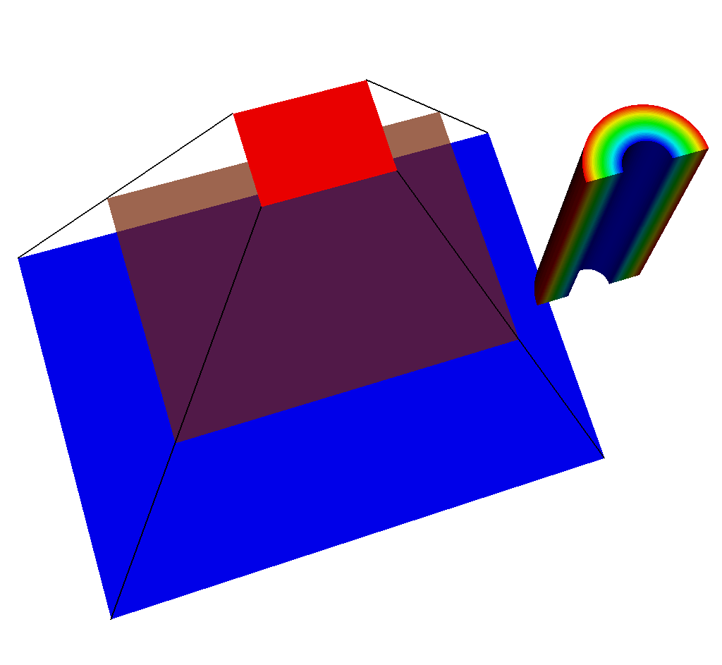
Fig. 8.58 An example of what could be going wrong. The simulated detector is not positioned correctly.

The simulated x ray detector is situated at the near plane, looking in the direction of the view plane, and seeing nothing after the far plane. Once the imaging planes and ray corners have been visualized, it is clear to see where the camera is looking, and if the near and far clipping planes are appropriately placed. See the text on visualizing the rays and imaging planes in Visualizing the Imaging Planes and Visualizing the Rays Meshes.

8.3.4.7.3. Where are the rays intersecting my geometry?

Answering this question is similarly simple. We will want to visualize the Rays Meshes on top of our input mesh.

# Make sure the mesh used in the query is already rendered.

# In this case, "output.root" is the name of the Blueprint file
# that was output from the query.
OpenDatabase("output.root")

# Add pseudocolor plots of each of the imaging planes.
# These help to add clarity to our final render.
AddPlot("Pseudocolor", "mesh_far_plane_topo/far_plane_field")
AddPlot("Pseudocolor", "mesh_view_plane_topo/view_plane_field")
AddPlot("Pseudocolor", "mesh_near_plane_topo/near_plane_field")

# Add a mesh plot of the rays.
AddPlot("Pseudocolor", "mesh_ray_topo/ray_field")

DrawPlots()

Running this code using VisIt should result in renders like those shown in Rays Meshes. Use the tips and tricks shown in that section to gain greater clarity for answering this question. See the text on visualizing the rays and imaging planes in Visualizing the Imaging Planes and Visualizing the Rays Meshes.

Fig. 8.59 An example render made using the above code.

8.3.4.7.4. What information is the query using to create the output?

See Accessing the Metadata for information on how to extract and view the Metadata, which contains all of the view parameters and query parameters that the query uses to create the output.

8.3.4.7.5. The fields in the Conduit Output are 1D. How can I reshape them to be 3D?

The following code examples will take resultant data (the intensity values, in this case) from the X Ray Image Query and reshape it to be 3D.

import conduit

def fetch_coordset_dims(data):
    cset_vals = data.fetch_existing("coordsets/image_coords/values")
    # fetch rectilinear coordset dims
    nx = cset_vals.fetch_existing("x").dtype().number_of_elements()
    ny = cset_vals.fetch_existing("y").dtype().number_of_elements()
    nz = cset_vals.fetch_existing("z").dtype().number_of_elements()
    # # if you would like to see the labels for these axes, this is
    # # how you can access them:
    # cset_lbls = data.fetch_existing("coordsets/image_coords/labels")
    # print(cset_lbls.fetch_existing("x"))
    # print(cset_lbls.fetch_existing("y"))
    # print(cset_lbls.fetch_existing("z"))
    return nx, ny, nz

def fetch_topology_dims(data):
    # rectilinear topology have one less element in each
    # logical dim than the coordset
    cnx, cny, cnz = fetch_coordset_dims(data)
    return cnx - 1, cny - 1, cnz - 1

def fetch_reshaped_field_values(data, field_name):
    nx, ny, nz = fetch_topology_dims(data)
    vals = data.fetch_existing("fields/" + field_name + "/values").value()
    return vals.reshape(nz, ny, nx)

We know that we should reshape in this order because x varies the fastest, then y, and then z. To verify this, we can examine the image_topo_order_of_domain_variables metadata (more information on that here: Other Metadata) which records in which order the axes vary. For the X Ray Image Query, this will always be x, then y, then z, so xrayout["domain_000000/state/xray_data/image_topo_order_of_domain_variables"] == "xyz" always.

Now that we have set everything up, let’s call the functions we created:

# read xray blueprint output
n = conduit.Node()

# the output file is in this case called "output.root"
conduit.relay.io.blueprint.load_mesh(n, "output.root")

# the node with our data is domain 0 -- or the first child
data = n[0] # the same could be done with data = 'n["domain_000000"]'

# the same could be done for "path_length"
intensity_vals = fetch_reshaped_field_values(data, "intensities")

print("1D intensities")
print(data["fields/intensities/values"])

print("3D intensity shape")
print(intensity_vals.shape)

print("3D intensities")
print(intensity_vals)

This produces the following:

1D intensities
[0.         0.         0.         0.         0.         0.20180537
 0.20180535 0.         0.         0.         0.         0.
 0.         0.         0.         0.         0.         0.20180537
 0.20180535 0.         0.         0.         0.         0.        ]

3D intensity shape
(2, 3, 4)

3D intensities
[[[0.         0.         0.         0.        ]
  [0.         0.20180537 0.20180535 0.        ]
  [0.         0.         0.         0.        ]]

 [[0.         0.         0.         0.        ]
  [0.         0.20180537 0.20180535 0.        ]
  [0.         0.         0.         0.        ]]]

The number of values is so small because I picked an image size of 4x3 pixels and 2 energy groups to demonstrate this.