8.5. Lineout
One-dimensional curves, created using data from 2D or 3D plots, are popular for analyzing data because they are simple to compare. VisIt’s visualization windows can be put into a mode that allows you to draw lines, along which data are extracted, in the visualization window. The extracted data are turned into a Curve plot in another visualization window. If no other visualization window exists, VisIt creates one and adds the Curve plot to it. Curve plots are often more useful than 2D Pseudocolor plots because they allow the data along a line to be seen spatially as a 1D curve instead of relying on differences in color to convey information. Furthermore, the curve data can be exported to curve files that allow the data to be imported into other Lawrence Livermore National Laboratory curve analysis software such as Ultra.
8.5.1. Lineout mode
You can put the visualization window into lineout mode by selecting the Lineout icon (Figure 8.63) in the visualization window’s Toolbar or from the Popup menu’s Mode submenu. Note that lineout mode is only available with 2D plots in this version though you can create 3D lineouts using the Lineout query in the Query Window. After the visualization window is in lineout mode, you can draw reference lines in the window. Each reference line causes VisIt to extract data from the database along the prescribed path and draw the data as a Curve plot in another visualization window. Each reference line is drawn in a color that matches the initial color of the Curve plot so the reference lines, which may not have labels, can be easily associated with their corresponding Curve plots. To clear the reference lines from the visualization window, select the Clear reference lines option from Popup menu’s Clear submenu. An example of the visualization window with reference lines and Curve plots is shown in Figure 8.64.

Fig. 8.63 Lineout mode toolbar icon
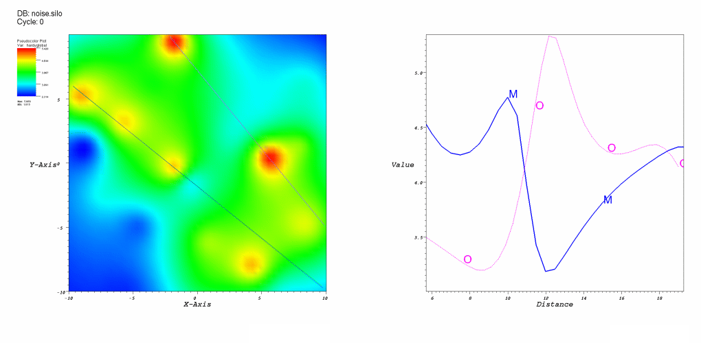
Fig. 8.64 Visualization windows with reference line and Curve plots
8.5.2. Curve plot
Curve plots are created by drawing reference lines. The visualization window must be in lineout mode before reference lines can be created. You can create a reference line by positioning the mouse over the first point of interest, clicking the left mouse button and then moving the mouse, while pressing the left mouse button, and releasing the mouse over the second endpoint. Releasing the mouse button creates a reference line along the path that was drawn with the mouse. When you draw a reference line, you cause a Curve plot of the data along the reference line to appear in another visualization window. If another visualization window is not available, VisIt opens a new one before creating the Curve plot. The Curve plot in the second window can be modified by setting the active window to the visualization window that contains the Curve plots.
See Curve Plot for information on changing the Curve plot’s appearance.
8.5.2.1. Saving curves
Once a curve has been generated, it can be saved to a curve file. A curve file is an ASCII text file that contains the X-Y pairs that make up the curve and it is useful for exporting curve data to other curve analysis programs. To save a curve, make sure you first set the active window to the visualization window that contains the curve. Next, save the window using the curve file format. All of the curves in the visualization window are saved to the specified curve file.
8.5.3. Lineout Operator
The Curve plot uses the Lineout operator to extract data from a database along a linear path. The Lineout operator is not generally available since curves are created only through reference lines and not the Plot menu. Still, once a curve has been created using the Lineout operator, certain attributes of the Lineout can be modified. Note that when you modify the Lineout attributes, it is best to turn off the Apply operators to all plots check box in the Main Window so that all curves do not get the same set of Lineout operator attributes.
There are two factors that affect how the interpolation along the line is performed. These are the centering of the variable and the lineout sampling method. There are two types of centering and two types of sampling. The following sections will go into detail for the four cases.
Zonal variables are constant within a cell and a lineout would be expected to be a step function as the line moves from cell to cell.
All the images associated with the examples can be generated with the script lineout.py.
8.5.3.1. Zonal centering with sampling
In the case of sampling, the step function will become more and more apparent as the number of sample points increases.
In the example below there are only 12 samples points and the step function is only somewhat apparent, since the number of sample points within a cell ranges between one and three.
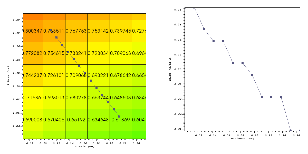
Fig. 8.65 A zonal variable with relatively few sample points.
In the example below there are 60 sample points and the step function is quite apparent.
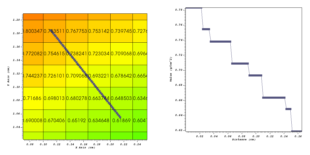
Fig. 8.66 A zonal variable with a large number of sample points.
8.5.3.2. Zonal centering without sampling
In the case of non-sampling, the sample points are chosen where the line intersects cell boundaries, which are lines in 2D and faces in 3D. The first point of the line has the zonal value of the cell it is within and the remaining points have the value of the cell the line is about to enter. In this case the step function nature of the variable is completely lost.
In the example below the sample points are placed based on where the line intersects the edges of the cells. The step function nature of the variable is completely lost and the line looks smoother than the sampled case.
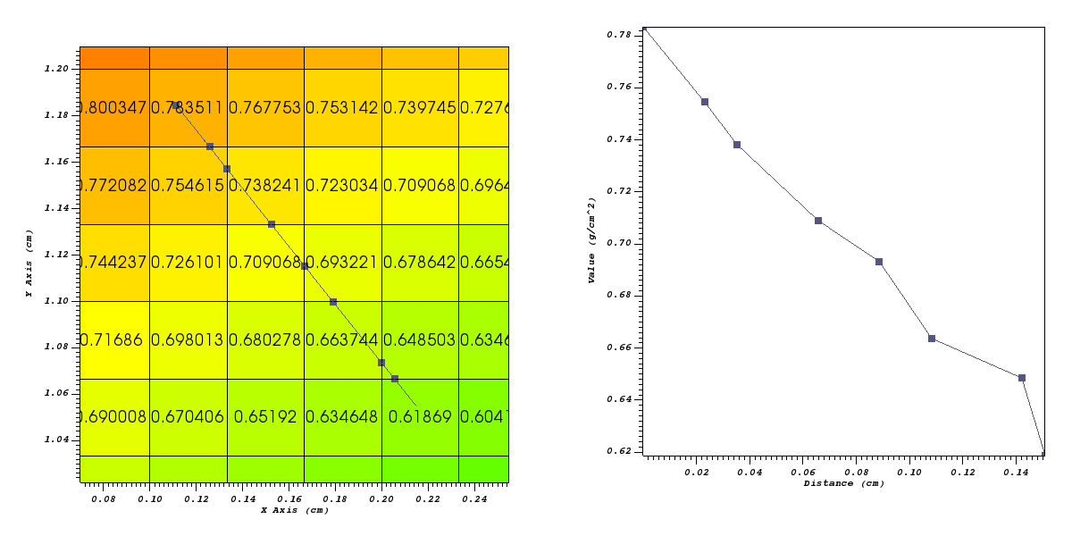
Fig. 8.67 A zonal variable without sampling.
Nodal variables vary linearly within a cell. Using sampling produces high quality results as long as the number of sample points is chosen such that all the cells along the line contain at least one sample point. Using non sampling tends to produce poor results based on its interpolation method (described below) and may result in jagged lines, even for smoothly varying functions.
8.5.3.3. Nodal centering with sampling
In the example below the 12 samples points do a good job of capturing the data along the line since all the cells are sampled at least once.

Fig. 8.68 A nodal variable with relatively few sample points.
Increasing the number of sample points in this case doesn’t change the shape of the curve.
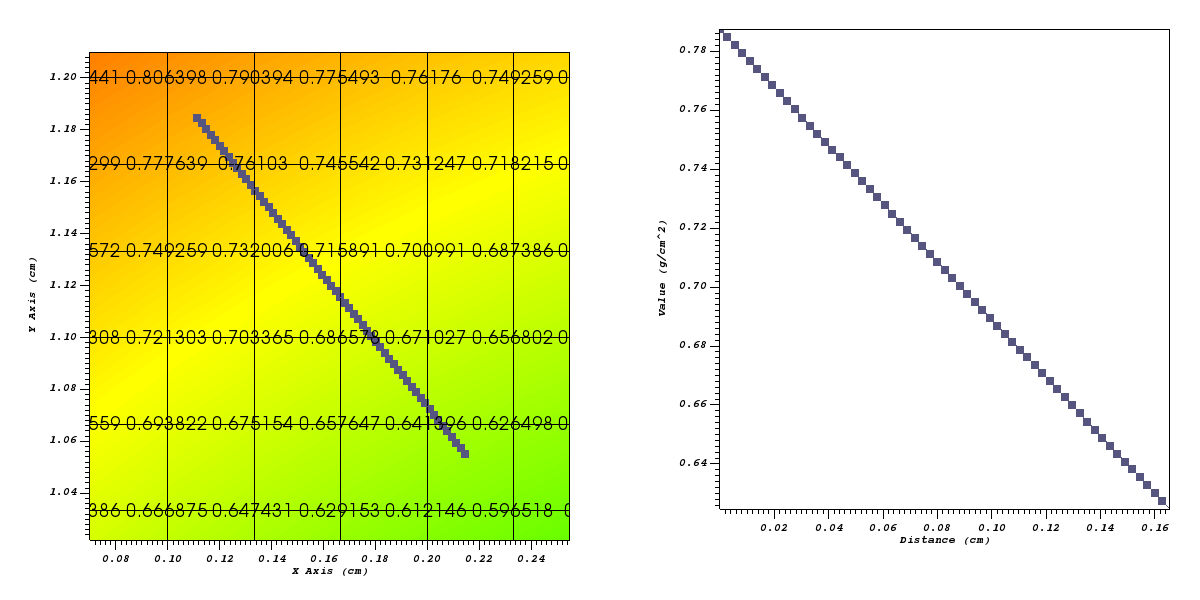
Fig. 8.69 A nodal variable with many sample points.
8.5.3.4. Nodal centering without sampling
In the example below the sample points are placed based on where the line intersects the edges of the cells. The first point of the line has the average of the nodes of the cell that the point is within and the remaining points have the value of the average of the nodes of the cell the line is about to enter. This can lead to a jagged line even for a smoothly varying function.
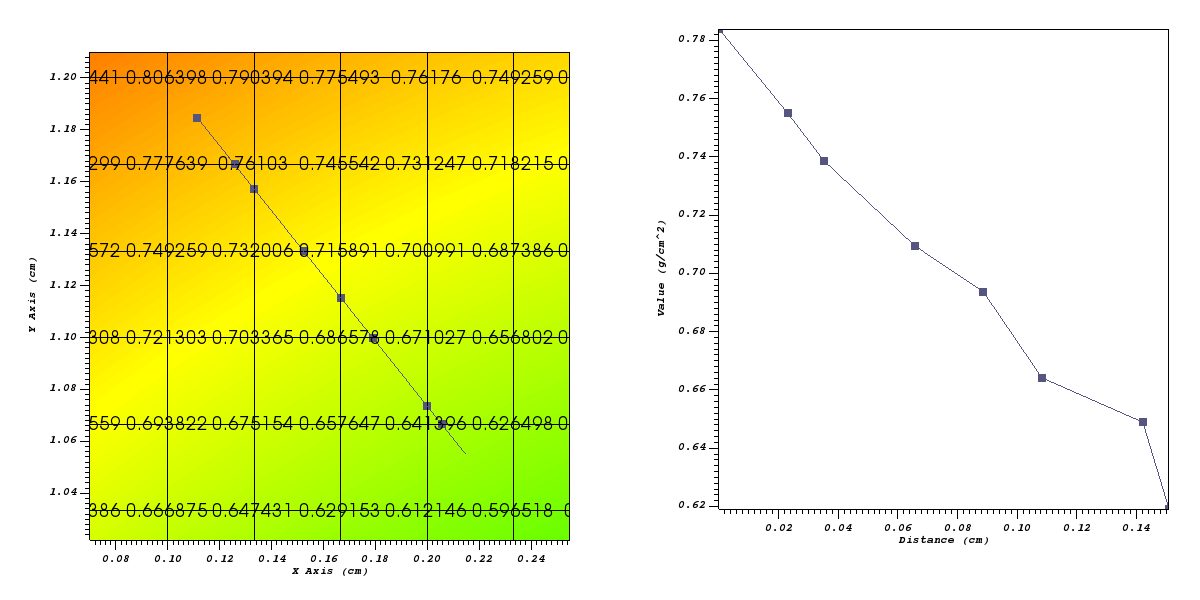
Fig. 8.70 A nodal variable without sampling.
8.5.3.5. Further exploring the Linout operator
The following script was used to generate 6 images above and can be used to further understand the behavior of the Lineout operator.
import math
import time

def create_images(sampling, n_samples, var):
    if (sampling == 1):
        save_name = "rect2d_%s_%d_lineout_sampled" % (var, n_samples)
        curve1_name = "rect2d_%s_%d_lineout_sampled.curve" % (var, n_samples)
        curve2_name = "rect2d_%s_%d_refline_sampled.curve" % (var, n_samples)
        image_name = "rect2d_%s_%d_pc_sampled" % (var, n_samples)
    else:
        save_name = "rect2d_%s_lineout_nonsampled" % var
        curve1_name = "rect2d_%s_lineout_nonsampled.curve" % var
        curve2_name = "rect2d_%s_refline_nonsampled.curve" % var
        image_name = "rect2d_%s_pc_nonsampled" % var

    #
    # Open the database to make the lineouts from.
    #
    OpenDatabase("rect2d.silo")

    #
    # Turn off extraneous annotations.
    #
    annot = AnnotationAttributes()
    annot.userInfoFlag = 0
    annot.databaseInfoFlag = 0
    annot.timeInfoFlag = 0
    annot.legendInfoFlag = 0
    SetAnnotationAttributes(annot)

    #
    # Create the lineout and do the lineout.
    #
    AddPlot("Mesh", "quadmesh2d")
    AddPlot("Pseudocolor", var)
    AddPlot("Label", var)
    labelAtts = LabelAttributes()
    labelAtts.numberOfLabels = 400
    SetPlotOptions(labelAtts)
    DrawPlots()
    view2D = View2DAttributes()
    view2D.windowCoords = (0.070, 0.255, 1.022, 1.210)
    view2D.viewportCoords = (0.15, 0.95, 0.1, 0.95)
    SetView2D(view2D)
    Lineout(start_point=(0.11137, 1.18468), end_point=(0.21461, 1.05520), use_sampling=sampling, num_samples=n_samples)

    #
    # Go to the lineout window, save the image, save the curve and create
    # a reference line with the sample points from the saved curve.
    #
    SetActiveWindow(2)
    SetAnnotationAttributes(annot)
    curveAtts = CurveAttributes()
    curveAtts.showPoints = 1
    curveAtts.pointSize = 8
    curveAtts.showLegend = 0
    curveAtts.showLabels = 0
    curveAtts.curveColorSource = curveAtts.Custom
    curveAtts.curveColor = (85, 85, 127, 255)
    SetPlotOptions(curveAtts)
    saveAtts = SaveWindowAttributes()
    saveAtts.fileName = save_name
    saveAtts.family = 0
    saveAtts.format = saveAtts.CURVE
    SetSaveWindowAttributes(saveAtts)
    SaveWindow()
    saveAtts.width = 600
    saveAtts.height = 600
    saveAtts.screenCapture = 0
    saveAtts.resConstraint = saveAtts.NoConstraint
    saveAtts.format = saveAtts.PNG
    SetSaveWindowAttributes(saveAtts)
    SaveWindow()

    #
    # Create a reference line with the sampled point from the saved curve
    # to overlay on the pseudocolor plot.
    #
    time.sleep(1)

    file1 = open(curve1_name, "r")
    file2 = open(curve2_name, "w")

    x1 = 0.11137
    y1 = 1.18468
    x2 = 0.21461
    y2 = 1.05520
    dx = x2 - x1
    dy = y2 - y1
    len = math.sqrt(dx * dx + dy * dy)
    dx = dx / len
    dy = dy / len
    slope = dy / dx

    line = file1.readline()
    line = file1.readline()
    file2.write("# refline\n")
    while line:
        vals = line.split()
        dist = float(vals[0])
        val = float(vals[1])
        x = x1 + (dist / len) * (x2 - x1)
        y = y1 + (dist / len) * (y2 - y1)
        file2.write("%g %g\n" % (x, y))
        line = file1.readline()

    file1.close()
    file2.close()

    time.sleep(1)

    #
    # Add the reference line to the pseudocolor plot.
    #
    SetActiveWindow(1)
    OpenDatabase(curve2_name)
    AddPlot("Curve", "refline")
    DrawPlots()
    SetPlotOptions(curveAtts)
    saveAtts.fileName = image_name
    SetSaveWindowAttributes(saveAtts)
    SaveWindow()

    #
    # Clean up.
    #
    DeleteAllPlots()
    SetActiveWindow(2)
    DeleteAllPlots()
    SetActiveWindow(1)
    CloseDatabase("rect2d.silo")
    CloseDatabase(curve2_name)

OpenComputeEngine("localhost", ("-np", "1"))

DefineScalarExpression("d2", "recenter(<d>, \"nodal\")")

create_images(1, 12, "d")
create_images(1, 60, "d")
create_images(0, 12, "d")
create_images(1, 12, "d2")
create_images(1, 60, "d2")
create_images(0, 12, "d2")

quit()
8.5.3.6. Setting lineout endpoints
You can modify the line endpoints by typing new coordinates into the Point 1 or Point 2 text fields of the Lineout attributes window (Figure 8.71). Each endpoint is a 3D coordinate that is specified by three space-separated floating point numbers. If you are performing a Lineout operation on 2D data, you can set the value for the Z coordinate to zero.
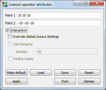
Fig. 8.71 Lineout attributes window
8.5.3.7. Setting the number of lineout samples
The sampling is controlled with the Use Sampling toggle button and the Samples text field. The Use Sampling toggle button controls whether sampling is used and Samples is used to set the number of sample points when sampling.
8.5.3.8. Interactive mode
When the Interactive check box is checked, changes to the Lineout operator can be made by using the Line tool available from the originating plot’s visualization window Toolbar or Popup menu. Interactive mode does not apply to lineouts created via the Curve plot’s variable menu,and the Line tool is disabled in such instances.
To utilize the line tool to modify a Lineout curve, make the visualization window with the originating plot the active window. Choose the Line tool. It should be initialized with the endpoints of the reference line. Moving the tool will change the lineout. See Interactive Tools for more information on tool utilization.
8.5.3.9. Reference line labels
You can make the reference lines in the window that caused Curve plots to be generated to have labels by checking the Lineout operator’s Refline Labels check box.
8.5.4. Lineout query
Performing a Lineout query requires an existing non-hidden plot in the active window. Choose Lineout from the Query window (available from the GUI’s Controls dropdown menu). Set start and end points (similar to Setting lineout endpoints). Lineout query is the only Lineout method that allows you to create curves for multiple variables. Simply select the desired variables from the Variables dropdown menu. Default means the variable as plotted in the currently active plot. A lineout curve will be generated for each variable, plotted along the same reference line. Each curve will have its own color. The Use Sampling and Sample Points option is the same as before.
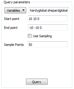
Fig. 8.72 Lineout query’s parameters window
8.5.5. Lineout via Curve plot variable menu
With this method, Lineout is considered one of the Operators that Generate New Variables. That means you can use it without first generating a plot of the data from which you wish to extract the lineout. To create a Lineout in this manner, open your database, select Curve plot, then choose operators/Lineout/<var-name> from the Curve plot’s variable menu as shown in Figure 8.73.
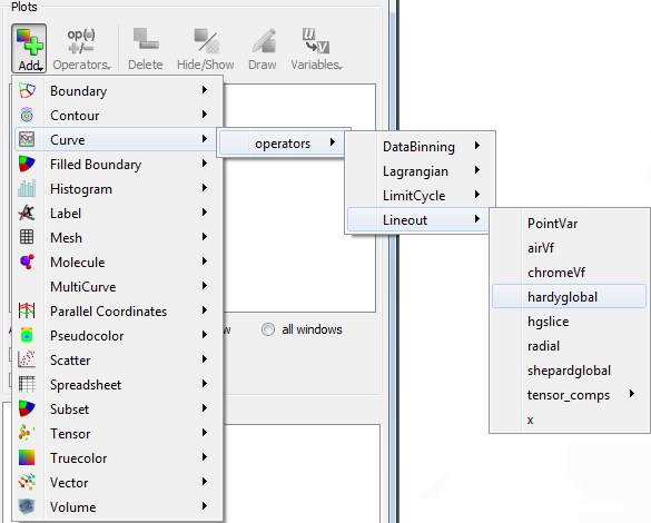
Fig. 8.73 Choosing lineout from the Curve plot’s variable menu
It is highly recommended that you modify the Lineout’s endpoints before clicking draw, as the defaults will probably not be appropriate for your data.
8.5.6. Global lineout options
The Lineout Options Window, available by selecting Lineout from the Controls menu in the Main Window contains global lineout options. They are global in the sense that they will apply to all future lineouts. The Lineout Options Window has controls for choosing the destination window of the lineout curve plots, as well as settings for how changes to the originating plot affect the lineout curve plot. Modifying these options will only apply to future lineouts, not lineouts already created.
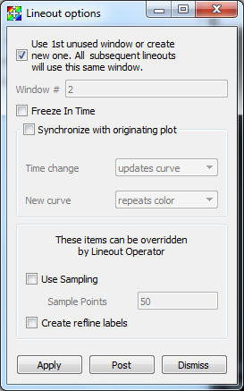
Fig. 8.74 Lineout Options Window
8.5.6.1. Lineout destination window
By default, VisIt will place all lineout curves in the same window. It will use the first unused open window or create one if one does not yet exist. You can override this behavior for future lineouts by unchecking the Use 1st unused window checkbox, and typing a window number into the Window # text box.
8.5.6.2. Freeze In Time
If the plot that originated the Lineout curve was from a time-varying database, the curve can be advanced in time using the animation controls for the window containing the lineout curve. If you would rather the lineout be frozen at the timestep from which it was taken, check the Freeze in Time option. This will also disable the ability to synchronize the lineout curve with its originating plot.
8.5.6.3. Synchronous lineout
Normally when you perform a lineout operation, the Curve plot that results from the lineout operation is in no way connected to the plots in the window that originated the Curve plot. If you want variable or timestate changes made to the originating plots to also affect the Curve plots that were created via lineout, click the Synchronize with originating plot check box in the Lineout Options Window (see Figure 8.74).
With this option selected, any change to the variable in the plot that originated the lineout, will update the lineout to reflect the new variable’s data. When you change timestates for the plot that originated the lineout, the lineout will update to reflect the data at the new timestate.
To make VisIt create a new Curve plot for the lineout instead of updating when you change timestates in the originating plot, change the Time change behavior in the Lineout Options Window from updates curve to creates new curve. VisIt will then put a new curve in the lineout destination window each time you advance to a new timestate, resulting in many Curve plots (see Figure 8.75). By default, VisIt will make all of the related Curve plots be the same color. You can override this behavior by selecting creates new color instead of repeats color from the New curve combo box.
Synchronization does not apply to lineout curves created via the Curve plot variable menu, as this type of lineout does not have an originating plot.
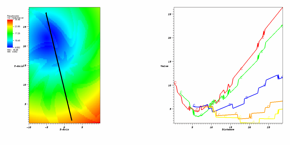
Fig. 8.75 Dynamic lineout can be used to create curves for multiple timestates
8.5.6.4. Sampling and Refline labels
These options are the same as described for individual lineouts. Use these options when you want your choices to apply to all lineouts.