3. Quick Recipes

3.1. Overview

This manual contains documentation for over two hundred functions and several dozen extension object types. Learning to combine the right functions in order to accomplish a visualization task without guidance would involve hours of trial and error. To maximize productivity and start creating visualizations using Visit’s Python Interface as fast as possible, this chapter provides some common patterns, or “quick recipes” that you can combine to quickly create complex scripts.

3.2. How to start

The most important question when developing a script is: “Where do I start?”. You can either use session files that you used to save the state of your visualization to initialize the plots before you start scripting or you can script every aspect of plot initialization.

3.2.1. Using session files

VisIt’s session files contain all of the information required to recreate plots that have been set up in previous interactive VisIt sessions. Since session files contain all of the information about plots, etc., they are natural candidates to make scripting easier since they can be used to do the hard part of setting up the complex visualization, leaving the bulk of the script to animate through time or alter the plots in some way. To use session files within a script, use the RestoreSession function.

# Import a session file from the current working directory. 
RestoreSession('/home/juan/visit/visit.session', 0) 
# Now that VisIt has restored the session, animate through time.
for state in range(TimeSliderGetNStates()): 
  TimeSliderSetState(state) 
  SaveWindow() 

3.2.2. Getting something on the screen

If you don’t want to use a session file to begin the setup for your visualization then you will have to dive into opening databases, creating plots, and animating through time. This is where all of hand-crafted scripts begin. The first step in creating a visualization is opening a database. VisIt provides the OpenDatabase function to open a database. Once a database has been opened, you can create plots from its variables using the AddPlot function. The AddPlot function takes a plot plugin name and the name of a variable from the open database. Once you’ve added a plot, it is in the new state, which means that it has not yet been submitted to the compute engine for processing. To make sure that the plot gets drawn, call the DrawPlots function.

# Step 1: Open a database 
OpenDatabase('~juanita/silo/stuff/wave.visit') 

# Step 2: Add plots with default properties
AddPlot('Pseudocolor', 'pressure') 
AddPlot('Mesh', 'quadmesh') 

# Step 3: Draw the plots with default view
DrawPlots() 

# Step 4: Iterate through time and save images 
for state in range(0,TimeSliderGetNStates(),10): 
  TimeSliderSetState(state) 
  SaveWindow() 

3.3. Using VisIt with the system Python

There are situations where you may want to import the VisIt module into the system Python. Some common use cases are using VisIt as part of a larger Python workflow or when you need to use a Python module that VisIt’s Python does not include. You should always try to use VisIt’s Python interpreter directly, since importing VisIt’s Python module may not always work.

When importing the VisIt module into the system Python, at a minimum the major version numbers must match and ideally the major and minor version numbers would match. In general, there are three things you must do to import the VisIt module into the system Python.

1. Tell the Python interpreter where the standard C++ library used to compile VisIt is located. This needs to be done before any modules other than ctypes are imported.

2. Tell the Python interpreter where the VisIt module is located.

3. Specify the version of VisIt you are using if you have multiple versions of VisIt installed in the same directory.

Not all of the steps are necessary. For example, if VisIt was compiled with the default system compiler then you do not need to perform the first step. It is important that the steps are done in the order specified above.

In this example VisIt is imported into the system Python and used to save an image from one of our sample datasets. The paths specified for the location of the standard C++ library and the VisIt module will need to be changed as appropriate for your system.

python3
Python 3.7.2 (default, Feb 26 2019, 08:59:10)
[GCC 4.9.3] on linux
Type "help", "copyright", "credits" or "license" for more information.
>>> import ctypes
>>> ctypes.cdll.LoadLibrary('/usr/tce/packages/gcc/gcc-7.3.0/lib64/libstdc++.so.6')
<CDLL '/usr/tce/packages/gcc/gcc-7.3.0/lib64/libstdc++.so.6', handle 6d3e30 at 0x2aaaac14b7f0>
>>> import sys
>>> sys.path.append("/usr/gapps/visit/3.3.3/linux-x86_64/lib/site-packages/")
>>> import visit
>>> visit.AddArgument("-v")
>>> visit.AddArgument("3.3.3")
>>> visit.LaunchNowin()
Running: viewer3.3.3 -nowin -forceversion 3.3.3 -noint -host 127.0.0.1 -port 5601
True
>>> import visit
>>> visit.OpenDatabase("/usr/gapps/visit/data/noise.silo")
Running: mdserver3.3.3 -forceversion 3.3.3 -host 127.0.0.1 -port 5601
Running: engine_ser3.3.3 -forceversion 3.3.3 -dir /usr/gapps/visit -idle-timeout 480 -host 127.0.0.1 -port 5601
1
>>> visit.AddPlot("Pseudocolor", "hardyglobal")
1
>>> visit.DrawPlots()
1
>>> visit.SaveWindow()
VisIt: Message - Rendering window 1...
VisIt: Message - Saving window 1...
VisIt: Message - Saved visit0000.png
'visit0000.png'
>>> quit()

Sometimes telling Python where the standard C++ library used to compile VisIt is located does not work and instead you can tell it where VisIt’s Python library is located.

python3
Python 3.9.12 (main, Apr 15 2022, 09:20:22)
[GCC 10.3.1 20210422 (Red Hat 10.3.1-1)] on linux
Type "help", "copyright", "credits" or "license" for more information.
>>> import ctypes
>>> ctypes.CDLL('/usr/gapps/visit/3.3.3/linux-x86_64-toss4/lib/libpython3.7m.so')
<CDLL '/usr/gapps/visit/3.3.3/linux-x86_64-toss4/lib/libpython3.7m.so', handle 508b30 at 0x155546edf4f0>
>>> import sys
>>> sys.path.append("/usr/gapps/visit/3.3.3/linux-x86_64-toss4/lib/site-packages")
>>> import visit
>>> visit.AddArgument("-v")
>>> visit.AddArgument("3.3.3")
>>> visit.LaunchNowin()
Running: viewer3.3.3 -nowin -forceversion 3.3.3 -noint -host 127.0.0.1 -port 5600
True
>>> import visit
>>> visit.OpenDatabase("/usr/gapps/visit/data/noise.silo")
Running: mdserver3.3.3 -forceversion 3.3.3 -host 127.0.0.1 -port 5600
Running: engine_ser3.3.3 -forceversion 3.3.3 -dir /usr/gapps/visit -idle-timeout 480 -host 127.0.0.1 -port 5600
1
>>> visit.AddPlot("Pseudocolor", "hardyglobal")
1
>>> visit.DrawPlots()
1
>>> visit.SaveWindow()
VisIt: Message - Rendering window 1...
VisIt: Message - Saving window 1...
VisIt: Message - Saved visit0000.png
'visit0000.png'
>>> quit()

3.4. Handling Command line arguments

In some cases, a VisIt python script also needs to handle its own command line arguments. This is handled using the Argv() method. For example, to run the python script, myscript.py with two arguments like so

visit -nowin -cli -s myscript.py myarg1 myarg2

these arguments can be accessed using the Argv() method which returns the Python tuple, ('myarg1', 'myarg2'). Similarly, sys.argv will return the Python list, ['myscript.py', 'myarg1', 'myarg2'] which includes the script name itself as the zeroth argument.

3.5. Saving images

Much of the time, the entire purpose of using VisIt’s Python Interface is to create a script that can save out images of a time-varying database for the purpose of making movies. Saving images using VisIt’s Python Interface is a straight-forward process, involving just a few functions.

3.5.1. Setting the output image characteristics

VisIt provides a number of options for saving files, including: format, fileName, and image width and height, to name a few. These attributes are grouped into the SaveWindowAttributes object. To set the options that VisIt uses to save files, you must create a SaveWindowAttributes object, change the necessary attributes, and call the SetSaveWindowAttributes function. Note that if you want to create images using a specific image resolution, the best way is to use the -geometry command line argument with VisIt’s Command Line Interface and tell VisIt to use screen capture. If you instead require your script to be capable of saving several different image sizes then you can turn off screen capture and set the image resolution in the SaveWindowAttributes object.

# Prepare to save a BMP file at 1024x768 resolution 
s = SaveWindowAttributes() 
s.format = s.BMP 
s.fileName = 'mybmpfile' 
s.width, s.height = 1024,768 
s.screenCapture = 0 
SetSaveWindowAttributes(s) 
# Subsequent calls to SaveWindow() will use these settings

3.5.2. Saving an image

Once you have set the SaveWindowAttributes to your liking, you can call the SaveWindow function to save an image. The SaveWindow function returns the name of the image that is saved so you can use that for other purposes in your script.

# Save images of all timesteps and add each image filename to a list.
names = []
for state in range(TimeSliderGetNStates()):
  SetTimeSliderState(state)
  # Save the image
  n = SaveWindow()
  names = names + [n]
print(names)

3.6. Working with databases

VisIt allows you to open a wide array of databases both in terms of supported file formats and in terms how databases treat time. Databases can have a single time state or can have multiple time states. Databases can natively support multiple time states or sets of single time states files can be grouped into time-varying databases using .visit files or using virtual databases. Working with databases gets even trickier if you are using VisIt to visualize a database that is still being generated by a simulation. This section describes how to interact with databases.

3.6.1. Opening a database

Opening a database is a relatively simple operation - most complexities arise in how the database treats time. If you only want to visualize a single time state or if your database format natively supports multiple timestates per file then opening a database requires just a single call to the OpenDatabase function.

# Open a database (no time specified defaults to time state 0)
OpenDatabase("/Users/amina/data/pdb_test_data/allinone00.pdb")

3.6.2. Opening a database at specific time

Opening a database at a later timestate is done just the same as opening a database at time state zero except that you must specify the time state at which you want to open the database. There are a number of reasons for opening a database at a later time state. The most common reason for doing so, as opposed to just changing time states later, is that VisIt uses the metadata from the first opened time state to describe the contents of the database for all timestates (except for certain file formats that don’t do this, i.e. SAMRAI). This means that the list of variables found for the first time state that you open is used for all timestates. If your database contains a variable at a later timestate that does not exist at earlier time states, you must open the database at a later time state to gain access to the transient variable.

# Open a database at a specific time state to pick up transient variables
OpenDatabase("/Users/amina/data/pdb_test_data/allinone00.pdb", 17)

3.6.3. Opening a virtual database

VisIt provides two ways for accessing a set of single time-state files as a single time- varying database. The first method is a .visit file, which is a simple text file that contains the names of each file to be used as a time state in the time-varying database. The second method uses “virtual databases”, which allow VisIt to exploit the file naming conventions that are often employed by simulation codes when they create their dumps. In many cases, VisIt can scan a specified directory and determine which filenames look related. Filenames with close matches are grouped as individual time states into a virtual database whose name is based on the more abstract pattern used to create the filenames.

# Opening just one file, the first, in series wave0000.silo, wave0010.silo, ...
OpenDatabase("~juanita/silo/stuff/wave0000.silo")

# Opening a virtual database representing all available states.
OpenDatabase("~juanita/silo/stuff/wave*.silo database")

3.6.4. Opening a remote database

VisIt supports running the client on a local computer while also allowing you to process data in parallel on a remote computer. If you want to access databases on a remote computer using VisIt’s Python Interface, the only difference to accessing a database on a local computer is that you must specify a host name as part of the database name.

# Opening a file on a remote computer by giving a host name
# Also, open the database to a later time slice (17)
OpenDatabase("thunder:~juanita/silo/stuff/wave.visit", 17)

3.7. Opening a compute engine

Sometimes it is advantageous to open a compute engine before opening a database. When you tell VisIt to open a database using the OpenDatabase function, VisIt also launches a compute engine and tells the compute engine to open the specified database. When the VisIt Python Interface is run with a visible window, the Engine Chooser Window will present itself so you can select a host profile. If you want to design a script that must specify parallel options, etc in batch mode where there is no Engine ChooserWindow then you have few options other than to open a compute engine before opening a database. To open a compute engine, use the OpenComputeEngine function. You can pass the name of the host on which to run the compute engine and any arguments that must be used to launch the engine such as the number of processors.

# Open a local, parallel compute engine before opening a database
# Use 4 processors on 2 nodes
OpenComputeEngine("localhost", ("-np", "4", "-nn", "2"))
OpenDatabase("~juanita/silo/stuff/multi_ucd3d.silo")

The options for starting the compute engine are the same as the ones used on the command line. Here are the most common options for launching a compute engine.

-l    <method>       Launch in parallel using the given method.
-np   <# procs>      The number of processors to use.
-nn   <# nodes>      The number of nodes to allocate.
-p    <part>         Partition to run in.
-b    <bank>         Bank from which to draw resources.
-t    <time>         Maximum job run time.
-machinefile <file>  Machine file.

The full list of parallel launch options can be obtained by typing visit --fullhelp. Here is a more complex example of launching a compute engine.

# Use the "srun" job launcher, the "batch" partition, the "mybank" bank,
# 72 processors on 2 nodes and a time limit of 1 hour
OpenComputeEngine("localhost",
    ("-l", "srun", "-p", "batch", "-b", "mybank",
     "-np", "72", "-nn", "2", "-t", "1:00:00"))

You can also launch a compute engine using one of the existing host profiles defined for your system. In this particular case we know that the second profile is for the “parallel” profile. If you didn’t know this you could print “p” to get all the properties.

# Set the user name to "user1" and use the 2nd profile,
# (indexed by 1 from zero) overriding a few of its properties
p = GetMachineProfile("quartz.llnl.gov")
p.userName="user1"
p.activeProfile = 1
p.GetLaunchProfiles(1).numProcessors = 6
p.GetLaunchProfiles(1).numNodes = 2
p.GetLaunchProfiles(1).timeLimit = "00:30:00"
OpenComputeEngine(p)

3.8. Working with plots

Plots are viewable objects, created from a database, that can be displayed in a visualization window. VisIt provides several types of plots and each plot allows you to view data using different visualization techniques. For example, the Pseudocolor plot allows you to see the general shape of a simulated object while painting colors on it according to the values stored in a variable’s scalar field. The most important functions for interacting with plots are covered in this section.

3.8.1. Creating a plot

The function for adding a plot in VisIt is: AddPlot. The AddPlot function takes the name of a plot type and the name of a variable that is to be plotted and creates a new plot and adds it to the plot list. The name of the plot to be created corresponds to the name of one of VisIt’s plot plugins, which can be queried using the PlotPlugins function. The variable that you pass to the AddPlot function must be a valid variable for the opened database. New plots are not realized, meaning that they have not been submitted to the compute engine for processing. If you want to force VisIt to process the new plot you must call the DrawPlots function.

# Names of all available plot plugins as a python tuple
x = PlotPlugins()

# print(x) will produce something like...
#     ('Boundary', 'Contour', 'Curve', 'FilledBoundary', 'Histogram',
#     'Label', 'Mesh', 'Molecule', 'MultiCurve', 'ParallelCoordinates',
#     'Pseudocolor', 'Scatter', 'Spreadsheet', 'Subset', 'Tensor',
#     'Truecolor', 'Vector', 'Volume')
print(x)

# Create plots with AddPlot(<plot-plugin-name>,<database-variable-name>)
AddPlot("Pseudocolor", "pressure")
AddPlot("Mesh", "quadmesh")

# Draw the plots
DrawPlots()

3.8.2. Plotting materials

Plotting materials is a common operation in VisIt. The Boundary and FilledBoundary plots enable you to plot material boundaries and materials, respectively.

# Plot material boundaries
AddPlot("Boundary", "mat1")
# Plot materials
AddPlot("FilledBoundary", "mat1")

3.8.3. Setting plot attributes

Each plot type has an attributes object that controls how the plot generates its data or how it looks in the visualization window. The attributes object for each plot contains different fields. You can view the individual object fields by printing the object to the console. Each plot type provides a function that creates a new instance of one of its attribute objects. The function name is always of the form: plotname + “Attributes”. For example, the attributes object creation function for the Pseudocolor plot would be: PseudocolorAttributes. To change the attributes for a plot, you create an attributes object using the appropriate function, set the properties in the returned object, and tell VisIt to use the new plot attributes by passing the object to the SetPlotOptions function. Note that you should set a plot’s attributes before calling the DrawPlots method to realize the plot since setting a plot’s attributes can cause the compute engine to recalculate the plot.

# Creating a Pseudocolor plot and setting min/max values.
AddPlot("Pseudocolor", "pressure")
p = PseudocolorAttributes()

# print p to find the names of members you want to change
#
# print(p) will produce output somewhat like...
#     scaling = Linear  # Linear, Log, Skew
#     skewFactor = 1
#     limitsMode = OriginalData  # OriginalData, ActualData
#     minFlag = 0
#     min = 0
#     useBelowMinColor = 0
#     belowMinColor = (0, 0, 0, 255)
#     maxFlag = 0
#     max = 1
#     .
#     .
#     .
print(p)

# Set the min/max values
p.min, p.minFlag = 0.0, 1
p.max, p.maxFlag = 10.0, 1
SetPlotOptions(p)

3.8.4. Working with multiple plots

When you work with more than one plot, it is sometimes necessary to set the active plots because some of VisIt’s functions apply to all of the active plots. The active plot is usually the last plot that was created unless you’ve changed the list of active plots. Changing which plots are active is useful when you want to delete or hide certain plots or set their plot attributes independently. When you want to set which plots are active, use the SetActivePlots function. If you want to list the plots that you’ve created, call the ListPlots function.

# Create more than 1 plot of the same type
AddPlot("Pseudocolor", "pressure")
AddPlot("Pseudocolor", "temperature")

# List the plots. The second plot should be active.
ListPlots()

# The output from ListPlots() will look something like...
#     Plot[0]|id=5;type="Pseudocolor";database="localhost:/Users/miller86/visit/visit/data/silo_hdf5_test_data/tire.silo";
#         var=pressure;active=0;hidden=0;framerange=(0, 0);keyframes={0};database keyframes={0};operators={};
#         activeOperator=-1
#     Plot[1]|id=6;type="Pseudocolor";database="localhost:/Users/miller86/visit/visit/data/silo_hdf5_test_data/tire.silo";
#         var=temperature;active=1;hidden=0;framerange=(0, 0);keyframes={0};database keyframes={0};operators={};
#         activeOperator=-1
# Note that active=1 for Plot[1] meaning plot #1 is the active plot

# Draw the plots
DrawPlots()

# Hide the first plot
SetActivePlots(0) # makes plot 0 the active plot
HideActivePlots()

# Set both plots' color table to "hot"
p = PseudocolorAttributes()
p.colorTableName = "hot"
SetActivePlots((0,1)) # makes both plots active
SetPlotOptions(p)

# Show the first plot again.
SetActivePlots(0)
HideActivePlots()

# Delete the second plot
SetActivePlots(1)
DeleteActivePlots()
ListPlots()

3.8.5. Plots in the error state

When VisIt’s compute engine cannot process a plot, the plot is put into the error state. Once a plot is in the error state, it no longer is displayed in the visualization window. If you are generating a movie, plots entering the error state can be a serious problem because you most often want all of the plots that you have created to animate through time and not disappear in the middle of the animation. You can add extra code to your script to prevent plots from disappearing (most of the time) due to error conditions by adding a call to the DrawPlots function.

# Open the database at state 20 and add plots for "pressure" and "transient".
# "transient" variable exists only in states 18...51.
OpenDatabase(silo_data_path("wave.visit"),20)
AddPlot("Pseudocolor","pressure")
AddPlot("Pseudocolor","transient")
DrawPlots()

# Start saving images from every 10th state starting at state 20 
# but take care to clean up when we get an error.
for state in range(20,TimeSliderGetNStates(),10):

    TimeSliderSetState(state)

    if DrawPlots() == 0:

        # Find plot(s) in error state and remove them
        pl = GetPlotList()
        for i in range(pl.GetNumPlots()):
            if pl.GetPlots(i).stateType == pl.GetPlots(i).Error:
                SetActivePlots((i,))
                DeleteActivePlots()

        # Clear the last error message
        GetLastError(1)

    SaveWindow()

3.9. Operators

Operators are filters that are applied to database variables before the compute engine uses them to create plots. Operators can be linked one after the other to form chains of operators that can drastically transform the data before plotting it.

3.9.1. Adding operators

The list of available operators is returned by the OperatorPlugins() function. Any of the names returned from OperatorPlugins() can be used to add an operator using the AddOperator() function. Adding an operator is similar to adding a plot in that you call a function with the name of the operator to be added. Operators are added only to the active plots by default but you can also force VisIt to add them to all plots in the plot list. You can also use the SetActivePlots() function to adjust the list of active plots before adding an operator to exercise finer grained control over which plots an operator is added to.

# Names of all available operator plugins as a python tuple
x = OperatorPlugins()

print(x)
# will produce output something like...
# ('AMRStitchCell', 'AxisAlignedSlice4D', 'BoundaryOp', 'Box', 'CartographicProjection',
#  'Clip', 'Cone', 'ConnectedComponents', 'CoordSwap', 'CreateBonds', 'Cylinder',
#  'DataBinning', 'DeferExpression', 'Displace', 'DualMesh', 'Edge', 'Elevate',
#  'EllipsoidSlice', 'Explode', 'ExternalSurface', ...
#  ..., 'TriangulateRegularPoints', 'Tube')

# We need at least one plot that we can add operators to
AddPlot("Pseudocolor", "dx")
AddPlot("Mesh","mesh1")

# Add Isovolume and Slice operators using whatever their default attributes are.
# The non-zero 2nd arg means to add the operator to all plots. If the 2nd argument
# is not present or zero, it means to add the operator only to the *active* plots
# (by default, the *active* plots are just the last plot added).
AddOperator("Isovolume", 1)
AddOperator("Slice", 1)
DrawPlots()

3.9.2. Setting operator attributes

Each plot gets its own instance of an operator which means that you can set each plot’s operator attributes independently. Like plots, operators use objects to set their attributes. These objects are returned by functions whose names are of the form: operatorname + “Attributes”. Once you have created an operator attributes object, you can pass it to the SetOperatorOptions to set the options for an operator. Note that setting the attributes for an operator nearly always causes the compute engine to recalculate the operator. You can use the power of VisIt’s Python Interface to create complex operator behavior such as in the following code example, which moves slice planes through a Pseudocolor plot.

OpenDatabase("~juanita/silo/stuff/noise.silo")
AddPlot("Pseudocolor", "hardyglobal")
AddOperator("Slice")
s = SliceAttributes()
s.originType = s.Percent
s.project2d = 0
SetOperatorOptions(s)
DrawPlots()

nSteps = 20
for axis in (0,1,2):
  s.axisType = axis
  for step in range(nSteps):
    t = float(step) / float(nSteps - 1)
    s.originPercent = t * 100.
    SetOperatorOptions(s)
    SaveWindow()

3.10. Quantitative operations

This section focuses on some of the operations that allow you to examine your data more quantitatively.

3.10.1. Defining expressions

VisIt allows you to create derived variables using its powerful expressions language. You can plot or query variables created using expressions just as you would if they were read from a database. VisIt’s Python Interface allows you to create new scalar, vector, tensor variables using the DefineScalarExpression, DefineVectorExpression, and DefineTensorExpression functions.

# Creating a new expression
OpenDatabase("~juanita/silo/stuff/noise.silo")
AddPlot("Pseudocolor", "hardyglobal")
DrawPlots()
DefineScalarExpression("newvar", "sin(hardyglobal) + cos(shepardglobal)")
ChangeActivePlotsVar("newvar")

3.10.2. Pick

VisIt allows you to pick on cells, nodes, and points within a database and return information for the item of interest. To that end, VisIt provides several pick functions. Once a pick function has been called, you can call the GetPickOutput function to get a string that contains the pick information. The information in the string could be used for a multitude of uses such as building a test suite for a simulation code.

OpenDatabase("~juanita/silo/stuff/noise.silo")
AddPlot("Pseudocolor", "hgslice")
DrawPlots()
s = []
# Pick by a node id
PickByNode(300)
s = s + [GetPickOutput()]
# Pick by a cell id
PickByZone(250)
s = s + [GetPickOutput()]
# Pick on a cell using a 3d point
Pick((-2., 2., 0.))
s = s + [GetPickOutput()]
# Pick on the node closest to (-2,2,0)
NodePick((-2,2,0))
s = s + [GetPickOutput()]
# Print all pick results
print(s)
# Will produce output somewhat like...
# ['\nA:  noise.silo\nMesh2D \nPoint: <-10, -7.55102>\nNode:...
#  '\nD:  noise.silo\nMesh2D \nPoint: <-1.83673, 1.83673>\nNode:...
#  ...\nhgslice:  <nodal> = 4.04322\n\n']

3.10.3. Lineout

VisIt allows you to extract data along a line, called a lineout, and plot the data using a Curve plot.

p0 = (-5,-3, 0)
p1 = ( 5, 8, 0)
OpenDatabase("~juanita/silo/stuff/noise.silo")
AddPlot("Pseudocolor", "hardyglobal")
DrawPlots()
Lineout(p0, p1)
# Specify 65 sample points
Lineout(p0, p1, 65)
# Do three variables ("default" is "hardyglobal")
Lineout(p0, p1, ("default", "airVf", "radial"))

The above steps produce the lineout(s), visually, as curve plot(s) in a new viewer window. Read more about how VisIt determines which window it uses for these curve plot(s). What if you want to access the actual lineout data and/or save it to a file?

# Set active window to one containing Lineout curve plots (typically #2)
SetActiveWindow(2)
# Get array of x,y pairs for first curve plot in window
SetActivePlots(0)
hg_vals = GetPlotInformation()["Curve"]
# Get array of x,y pairs for second curve plot in window
SetActivePlots(1)
avf_vals = GetPlotInformation()["Curve"]
# Get array of x,y pairs for third curve plot in window
SetActivePlots(2)
rad_vals = GetPlotInformation()["Curve"]

# Write it as CSV data to a file
for i in range(int(len(hg_vals) / 2)):
    idx = i*2+1 # take only y-values in each array
    print("%g,%g,%g" % (hg_vals[idx], avf_vals[idx], rad_vals[idx]))

3.10.4. Query

VisIt can perform a number of different queries based on values calculated about plots or their originating database.

OpenDatabase("~juanita/silo/stuff/noise.silo")
AddPlot("Pseudocolor", "hardyglobal")
DrawPlots()
Query("NumNodes")
print("The float value is: %g" % GetQueryOutputValue())
Query("NumNodes")

3.10.5. Finding the min and the max

A common operation in debugging a simulation code is examining the min and max values. Here is a pattern that allows you to print out the min and the max values and their locations in the database and also see them visually.

# Define a helper function to get node/zone id's from query string.
def GetMinMaxIds(qstr):
    import string
    s = qstr.split(' ')
    retval = []
    nextGood = 0
    idType = 0
    for token in s:
        if token == "(zone" or token == "(cell":
            idType = 1
            nextGood = 1
            continue
        elif token == "(node":
            idType = 0
            nextGood = 1
            continue
        if nextGood == 1:
            nextGood = 0
            retval = retval + [(idType, int(token))]
    return retval

# Set up a plot
OpenDatabase("~juanita/silo/stuff/noise.silo")
AddPlot("Pseudocolor", "hgslice")
DrawPlots()
Query("MinMax")

# Do picks on the ids that were returned by MinMax.
for ids in GetMinMaxIds(GetQueryOutputString()):
    idType = ids[0]
    id = ids[1]
    if idType == 0:
        PickByNode(id)
    else:
        PickByZone(id)

Note that the above example parses information from the query output string returned from GetQueryOutputString(). In some cases, it will be more convenient to use GetQueryOutputValue() or GetQueryOutputObject().

3.10.6. Creating a CSV file of a query over time

VisIt has the ability to perform queries over time to create one or more curves. It generates one curve per scalar value returned by the query. Frequently, the user wants to process the result of a query over time. A CSV file is a convenient way to output the data for further processing.

Here is a pattern where we loop over the time steps writing the results of a Time query and a PickByNode to a text file in the form of a CSV file.

OpenDatabase("~juanita/silo/stuff/wave.visit")
AddPlot("Pseudocolor", "pressure")
DrawPlots()

n_time_steps = TimeSliderGetNStates()
f = open('points.txt', 'w', encoding='utf-8')
f.write('time, x, y, z, u, v, w\n')
for time_step in range(0, n_time_steps):
    TimeSliderSetState(time_step)
    pick = PickByNode(domain=0, element=3726, vars=["u", "v", "w"])
    Query("Time")
    time = GetQueryOutputValue()
    f.write('%g, %g, %g, %g, %g, %g, %g\n' % (time, pick['point'][0], pick['point'][1], pick['point'][2], pick['u'], pick['v'], pick['w']))
f.close()

You can substitute the Time and PickByNode queries with your favorite query, such as the MinMax query used in the previous quick recipe.

3.11. Subsetting

VisIt allows the user to turn off subsets of the visualization using a number of different methods. Databases can be divided up any number of ways: domains, materials, etc. This section provides some details on how to remove materials and domains from your visualization.

3.11.1. Turning off domains

VisIt’s Python Interface provides the TurnDomainsOn and TurnDomainsOff functions to make it easy to turn domains on and off.

OpenDatabase("~juanita/silo/stuff/multi_rect2d.silo")
AddPlot("Pseudocolor", "d")
DrawPlots()

# Turning off every other domain
d = GetDomains()
i = 0
for dom in d:
    if i%2:
        TurnDomainsOff(dom)
    i += 1

# Turn all domains off
TurnDomainsOff()

# Turn on domains 3,5,7
TurnDomainsOn((d[3], d[5], d[7]))

3.11.2. Turning off materials

VisIt’s Python Interface provides the TurnMaterialsOn and TurnMaterialsOff functions to make it easy to turn materials on and off.

OpenDatabase("~juanita/silo/stuff/multi_rect2d.silo")
AddPlot("FilledBoundary", "mat1")
DrawPlots()
# Get the material names 
GetMaterials()
# GetMaterials() will return a tuple of material names such as
#     ('1', '2', '3')
# Turn off material with name "2"
TurnMaterialsOff("2")

3.12. View

Setting up the view in your Python script is one of the most important things you can do to ensure the quality of your visualization because the view concentrates attention on an object of interest. VisIt provides different methods for setting the view, depending on the dimensionality of the plots in the visualization window but despite differences in how the view is set, the general procedure is basically the same.

3.12.1. Setting the 2D view

The 2D view consists of a rectangular window in 2D space and a 2D viewport in the visualization window. The window in 2D space determines what parts of the visualization you will look at while the viewport determines where the images will appear in the visualization window. It is not necessary to change the viewport most of the time.

OpenDatabase("~juanita/silo/stuff/noise.silo")
AddPlot("Pseudocolor", "hgslice")
AddPlot("Mesh", "Mesh2D")
AddPlot("Label", "hgslice")
DrawPlots()
print("The current view is:", GetView2D())
# Get an initialized 2D view object.
# Note that DrawPlots() must be executed prior to getting
# the view to ensure current view parameters are obtained
v = GetView2D()
v.windowCoords = (-7.67964, -3.21856, 2.66766, 7.87724)
SetView2D(v)

3.12.2. Setting the 3D view

The 3D view is much more complex than the 2D view. For information on the actual meaning of the fields in the View3DAttributes object, refer to page 214 or the VisIt User Manual. VisIt automatically computes a suitable view for 3D objects and it is best to initialize new View3DAttributes objects using the GetView3D function so most of the fields will already be initialized. The best way to get new views to use in a script is to interactively create the plot and repeatedly call GetView3D() after you finish rotating the plots with the mouse. You can paste the printed view information into your script and modify it slightly to create sophisticated view transitions.

OpenDatabase("~juanita/silo/stuff/noise.silo")
AddPlot("Pseudocolor", "hardyglobal")
AddPlot("Mesh", "Mesh")
DrawPlots()
# Note that DrawPlots() must be executed prior to getting
# the view to ensure current view parameters are obtained
v = GetView3D()
print("The view is: ", v)
v.viewNormal = (-0.571619, 0.405393, 0.713378)
v.viewUp = (0.308049, 0.911853, -0.271346)
SetView3D(v)

3.12.3. Flying around plots

Flying around plots is a commonly requested feature when making movies. Fortunately, this is easy to script. The basic method used for flying around plots is interpolating the view. VisIt provides a number of functions that can interpolate View2DAttributes and View3DAttributes objects. The most useful of these functions is the EvalCubicSpline function. The EvalCubicSpline function uses piece-wise cubic polynomials to smoothly interpolate between a tuple of N like items. Scripting smooth view changes using EvalCubicSpline is rather like keyframing in that you have a set of views that are mapped to some distance along the parameterized space [0., 1.]. When the parameterized space is sampled with some number of samples, VisIt calculates the view for the specified parameter value and returns a smoothly interpolated view. One benefit over keyframing, in this case, is that you can use cubic interpolation whereas VisIt’s keyframing mode currently uses linear interpolation.

OpenDatabase("~juanita/silo/stuff/globe.silo")
AddPlot("Pseudocolor", "u")
DrawPlots()

# Create the control points for the views.
c0 = View3DAttributes()
c0.viewNormal = (0, 0, 1)
c0.focus = (0, 0, 0)
c0.viewUp = (0, 1, 0)
c0.viewAngle = 30
c0.parallelScale = 17.3205
c0.nearPlane = 17.3205
c0.farPlane = 81.9615
c0.perspective = 1

c1 = View3DAttributes()
c1.viewNormal = (-0.499159, 0.475135, 0.724629)
c1.focus = (0, 0, 0)
c1.viewUp = (0.196284, 0.876524, -0.439521)
c1.viewAngle = 30
c1.parallelScale = 14.0932
c1.nearPlane = 15.276
c1.farPlane = 69.917
c1.perspective = 1

c2 = View3DAttributes()
c2.viewNormal = (-0.522881, 0.831168, -0.189092)
c2.focus = (0, 0, 0)
c2.viewUp = (0.783763, 0.556011, 0.27671)
c2.viewAngle = 30
c2.parallelScale = 11.3107
c2.nearPlane = 14.8914
c2.farPlane = 59.5324
c2.perspective = 1

c3 = View3DAttributes()
c3.viewNormal = (-0.438771, 0.523661, -0.730246)
c3.focus = (0, 0, 0)
c3.viewUp = (-0.0199911, 0.80676, 0.590541)
c3.viewAngle = 30
c3.parallelScale = 8.28257
c3.nearPlane = 3.5905
c3.farPlane = 48.2315
c3.perspective = 1

c4 = View3DAttributes()
c4.viewNormal = (0.286142, -0.342802, -0.894768)
c4.focus = (0, 0, 0)
c4.viewUp = (-0.0382056, 0.928989, -0.36813)
c4.viewAngle = 30
c4.parallelScale = 10.4152
c4.nearPlane = 1.5495
c4.farPlane = 56.1905
c4.perspective = 1

c5 = View3DAttributes()
c5.viewNormal = (0.974296, -0.223599, -0.0274086)
c5.focus = (0, 0, 0)
c5.viewUp = (0.222245, 0.97394, -0.0452541)
c5.viewAngle = 30
c5.parallelScale = 1.1052
c5.nearPlane = 24.1248
c5.farPlane = 58.7658
c5.perspective = 1

# Make the last point loop around to the first
c6 = c0

# Create a tuple of camera values and x values. The x values
# determine where in [0,1] the control points occur.
cpts = (c0, c1, c2, c3, c4, c5, c6)
x=[]
for i in range(7):
    x = x + [float(i) / float(6.)]

# Animate the view using EvalCubicSpline.
nsteps = 100
for i in range(nsteps):
    t = float(i) / float(nsteps - 1)
    c = EvalCubicSpline(t, x, cpts)
    c.nearPlane = -34.461
    c.farPlane = 34.461
    SetView3D(c)

3.13. Working with annotations

Adding annotations to your visualization improve the quality of the final visualization in that you can refine the colors that you use, add logos, or highlight features of interest in your plots. This section provides some recipes for creating annotations using scripting.

3.13.1. Using gradient background colors

VisIt’s default white background is not necessarily the best looking background color for presentations. Adding a gradient background under your plots is an easy way to add a small professional touch to your visualizations. VisIt provides a few different styles of gradient background: radial, top to bottom, bottom to top, left to right, and right to left. The gradient style is set using the gradientBackgroundStyle member of the AnnotationAttributes object. The before and after results are shown in Figure 3.67.

# Set a blue/black, radial, gradient background.
a = AnnotationAttributes()
a.backgroundMode = a.Gradient
a.gradientBackgroundStyle = a.Radial
a.gradientColor1 = (0,0,255,255) # Blue
a.gradientColor2 = (0,0,0,255) # Black
SetAnnotationAttributes(a)

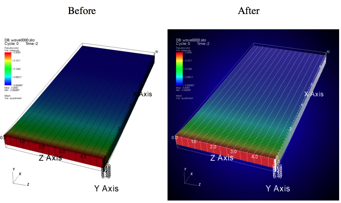
Fig. 3.67 Before and after image of adding a gradient background.

3.13.2. Adding a banner

Banners are useful for providing titles for a visualization or for marking its content (see Figure 3.68). To add an “Unclassified” banner to a visualization, use the following bit of Python code:

# Create a Text2D object to indicate the visualization is unclassified.

# Note the annoation object is added to the viewer window the moment it is created.
banner = CreateAnnotationObject("Text2D")

# Note text is updated in the viewer window the moment it is changed.
banner.text = "Unclassified"

banner.position = (0.37, 0.95)
banner.fontBold = 1

# print the attributes to see what you can set in the Text2D object.
print(banner)
# print(banner) will print something like...
#    visible = 1
#    position = (0.5, 0.5)
#    height = 0.03
#    textColor = (0, 0, 0, 255)
#    useForegroundForTextColor = 1
#    text = "2D text annotation"
#    fontFamily = Arial  # Arial, Courier, Times
#    fontBold = 0
#    fontItalic = 0
#    fontShadow = 0

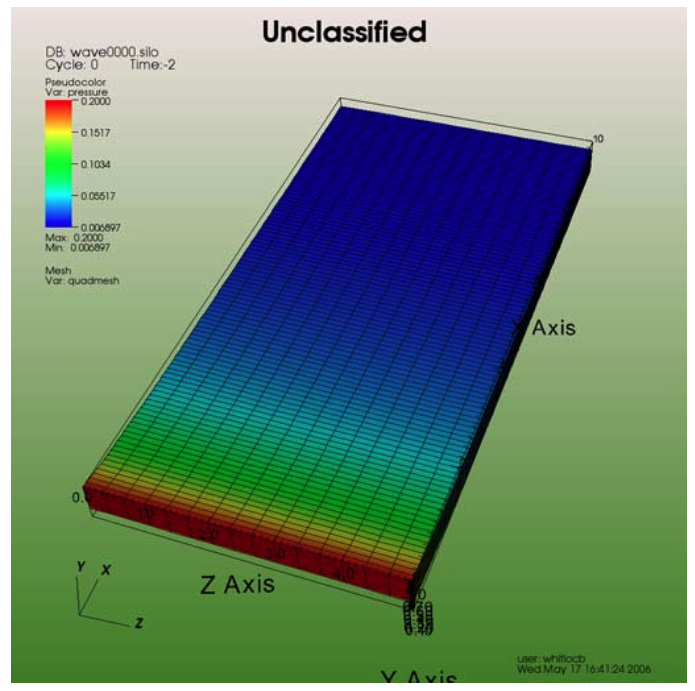
Fig. 3.68 Adding a banner

3.13.3. Adding a time slider

Time sliders are important annotations for movies since they convey how much progress an animation has made as well as how many more frames have yet to be seen. The time slider is also important for showing the simulation time as the animation progresses so users can get a sense of when in the simulation important events occur. VisIt’s time slider annotation object is shown in Figure 3.69.

# Add a time slider in the lower left corner
slider = CreateAnnotationObject("TimeSlider")

# Adjust the height. Takes effect immediately as the value is assigned.
slider.height = 0.07

# Print members that are available in the time slider object
print(slider)
# will produce something like...
#    visible = 1
#    active = 1
#    position = (0.01, 0.01)
#    width = 0.4
#    height = 0.05
#    textColor = (0, 0, 0, 255)
#    useForegroundForTextColor = 1
#    startColor = (0, 255, 255, 255)
#    endColor = (255, 255, 255, 153)
#    text = "Time=$time"
#    timeFormatString = "%g"
#    timeDisplay = AllFrames  # AllFrames, FramesForPlot, StatesForPlot, UserSpecified
#    percentComplete = 0
#    rounded = 1
#    shaded = 1

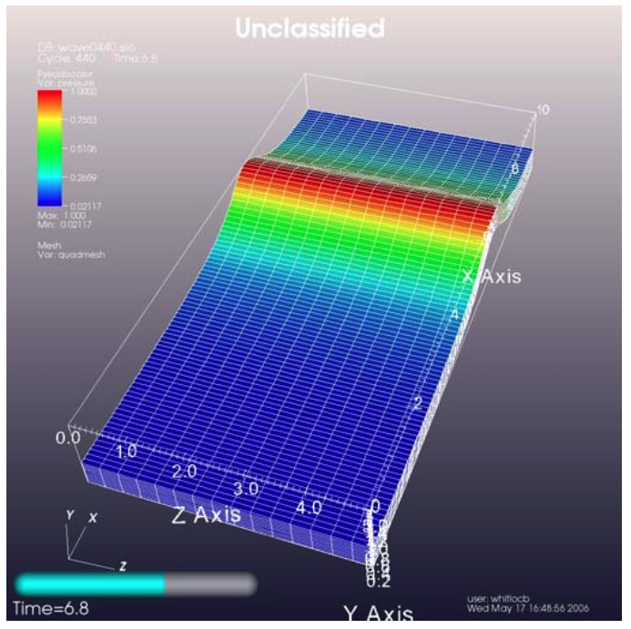
Fig. 3.69 Time slider annotation in the lower left corner

3.13.4. Adding a logo

Adding a logo to a visualization is an important part of project identification for movies and other visualizations created with VisIt. If you have a logo image file stored in TIFF, JPEG, BMP, or PPM format then you can use it with VisIt as an image annotation (see Figure 3.70). Note that this approach can also be used to insert images of graphs, plots, portraits, diagrams, or any other form of image data into a visualization.

# Incorporate LLNL logo image (llnl.jpeg) as an annotation
image = CreateAnnotationObject("Image")
image.image = "llnl.jpeg"
image.position = (0.02, 0.02)

# Print the other image annotation options
print(image)
# Will print something like...
#    visible = 1
#    active = 1
#    position = (0, 0)
#    transparencyColor = (0, 0, 0, 255)
#    useTransparencyColor = 0
#    width = 100.000000
#    height = 100.000000
#    maintainAspectRatio = 1
#    image = ("")

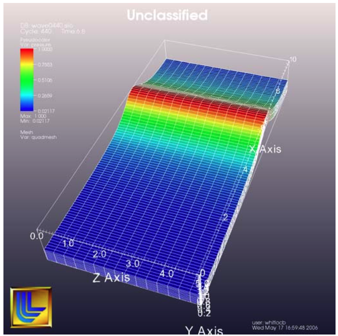
Fig. 3.70 Image annotation used to incorporate LLNL logo

3.13.5. Modifying a legend

VisIt’s plot legends can be customized. To obtain the proper annotation object, you must use the name of the plot, which is a unique name that identifies the plot. Once you have the plot’s name, you can obtain a reference to its legend annotation object and start setting properties to modify the legend.

# Open a file and make a plot
OpenDatabase("~juanita/silo/stuff/noise.silo")
AddPlot("Mesh", "Mesh")
AddPlot("Pseudocolor", "hardyglobal")
DrawPlots()
# Get the legend annotation object for the Pseudocolor plot, the second
# plot in the list (0-indexed).
plotName = GetPlotList().GetPlots(1).plotName
legend = GetAnnotationObject(plotName)
# See if we can scale the legend.
legend.xScale = 3.
legend.yScale = 3.
# the bounding box.
legend.drawBoundingBox = 1
legend.boundingBoxColor = (180,180,180,230)
# Make it horizontal
legend.orientation = legend.HorizontalBottom
# moving the legend
legend.managePosition = 0
legend.position = (0.7,0.15)
# text color
InvertBackgroundColor()
legend.useForegroundForTextColor = 0
legend.textColor = (255, 0, 0, 255)
# number format
legend.numberFormat = "%1.4e"
# the font.
legend.fontFamily = legend.Arial
legend.fontBold = 1
legend.fontItalic = 1
# turning off the labels.
legend.fontItalic = 0
legend.drawLabels = 0
legend.drawMinMax = 0
# turning off the title.
legend.drawTitle = 0
# Use user-supplied labels, rather than numeric values.
legend.controlTicks=0
legend.drawLabels = legend.Labels
# suppliedLabels must be strings, only valid when controlTicks is 0
legend.suppliedLabels=("A", "B", "C", "D", "E")
# Give the legend a custom title
legend.useCustomTitle=1
legend.customTitle="my custom title"

3.14. Working with color tables

Sometimes it is helpful to create a new color table or manipulate an existing user defined color table. Color tables consist of ControlPoints which specify color and position in the color spectrum as well as a few other standard options.

Existing color tables can be retreived by name via GetColorTable as in:

hotCT = GetColorTable("hot")
print(hotCT)
# results of print
#    GetControlPoints(0).colors = (0, 0, 255, 255)
#    GetControlPoints(0).position = 0
#    GetControlPoints(1).colors = (0, 255, 255, 255)
#    GetControlPoints(1).position = 0.25
#    GetControlPoints(2).colors = (0, 255, 0, 255)
#    GetControlPoints(2).position = 0.5
#    GetControlPoints(3).colors = (255, 255, 0, 255)
#    GetControlPoints(3).position = 0.75
#    GetControlPoints(4).colors = (255, 0, 0, 255)
#    GetControlPoints(4).position = 1
#    smoothing = Linear  # NONE, Linear, CubicSpline
#    equalSpacingFlag = 0
#    discreteFlag = 0

The colors field of the ControlPoint represent the (Red,Green,Blue,Alpha) channels of the color and must be in the range (0, 255). The numbers indicate the contribution each channel makes to the overall color. Higher values mean higher saturation of the color. For example, red would be represented as (255, 0, 0, 255), while yellow would be (255, 255, 0, 255), an equal combination of red and green. Playing with the Color selection dialog from the Popup color menu in the gui can help in determining RGBA values for desired colors. See Figure 9.10.

Alpha indicates the level of transparency of the color, with a value of 255 meaning fully opaque, and 0, fully transparent. Not all plots in VisIt make use of the Alpha channel of a color table. For instance, for Pseudocolor plots, one must set the opacityType to ColorTable in order for a Color table with semi-transparent colors to have any effect.

The position field of the ControlPoint is in the range (0, 1) and should be in ascending order.

General information on VisIt’s color tables can be found in the Color Tables section of Using VisIt.

In all the examples below, silo_data_path() refers to a function specific to VisIt testing that returns the path to silo example data. When copying the examples don’t forget to modify that reference according to your needs.

3.14.1. Modifying existing color tables

User-defined color tables can be modified by Adding or Removing ControlPoints, and by changing ControlPoint colors and position:

OpenDatabase(silo_data_path("rect2d.silo"))
AddPlot("Pseudocolor", "d")

pc = PseudocolorAttributes()
pc.centering=pc.Nodal 
# set color table name
pc.colorTableName = "hot"
SetPlotOptions(pc)

DrawPlots()
# put the plot in full-frame mode
v = GetView2D()
v.fullFrameActivationMode= v.On
SetView2D(v)

hotCT = GetColorTable("hot")

# Remove a couple of control points
hotCT.RemoveControlPoints(4)
hotCT.RemoveControlPoints(3)

# We must use a different name, as VisIt will not allow overwriting of built-in color tables
SetColorTable("hot_edited", hotCT)

# set color table name so changes to it will be reflected in plot
pc.colorTableName = "hot_edited"
SetPlotOptions(pc)

# Change colors
hotCT.GetControlPoints(0).colors = (255,0,0,255)
hotCT.GetControlPoints(1).colors = (255, 0, 255, 255)
SetColorTable("hot_edited", hotCT)

# Turn on equal spacing
hotCT.equalSpacingFlag = 1
# Create a new color table by providing a different name
SetColorTable("hot2", hotCT)

# tell the Pseudocolor plot to use the new color table
pc.colorTableName = "hot2"
SetPlotOptions(pc)

# Change positions so that the first and last are at the endpoints
hotCT.equalSpacingFlag=0
hotCT.GetControlPoints(0).position = 0
hotCT.GetControlPoints(1).position =0.5 
hotCT.GetControlPoints(2).position = 1
SetColorTable("hot3", hotCT)

pc.colorTableName = "hot3"
SetPlotOptions(pc)

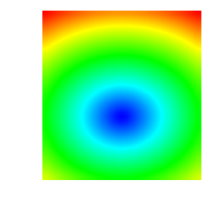
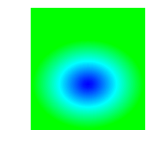
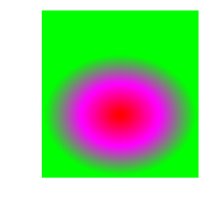
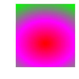
In the set of images below we can see how the plot changes as the color table it uses is modified: with original ‘hot’ color table; after removing control points; after changing colors; after using equal spacing and after changing positions.

3.14.2. Creating a continous color table from scratch

Creating a continuous color table involves creating a ColorControlPoint for each color you want, setting its colors and position fields and then adding them to a ColorControlPointList. The ColorControlPointList is then passed as an argument to AddColorTable.

# create control points (red, green, blue, position).
ct = ((1,0,0,0.), (1,0.8,0.,0.166), (1,1,0,0.333), (0,1,0,0.5),
      (0,1,1,0.666), (0,0,1,0.8333), (0.8,0.1,1,1))

ccpl = ColorControlPointList()

# add the control points to the list 
for pt in ct:
    p = ColorControlPoint()
    # colors is RGBA and must be in range 0...255
    p.colors = (pt[0] * 255, pt[1] * 255, pt[2] * 255, 255)
    p.position = pt[3]
    ccpl.AddControlPoints(p)
AddColorTable("myrainbow", ccpl)

OpenDatabase(silo_data_path("globe.silo"))
AddPlot("Pseudocolor", "speed")

# Make the plot use the new color table
pc = PseudocolorAttributes(1)
pc.colorTableName = "myrainbow"
SetPlotOptions(pc)

DrawPlots()

v = GetView3D()
v.viewNormal = (-0.693476, 0.212776, 0.688344)
v. viewUp = (0.161927, 0.976983, -0.138864)
SetView3D(v)

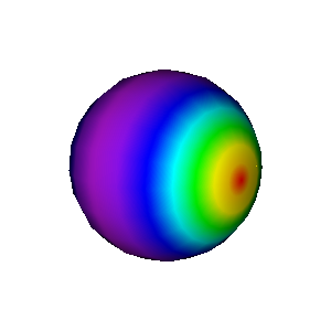
Fig. 3.71 Pseudocolor plot resulting from using the “myrainbow” color table.

3.14.3. Creating a discrete color table from scratch

Sometimes you may not want to figure out RGBA values for colors you want to use. In that case you can import a color module that will give you the RGBA values for named colors that are part of the module. Here’s an example of creating a discrete color table using named colors from the vtk module:

try:
    import vtk # for vtk.vtkNamedColors
except:
    return

# to see list of all color names available: 
# print(vtk.vtkNamedColors.GetColorNames())

# choose some colors from vtk.vtkNamedColors
colorNames = ["tomato", "turquoise", "van_dyke_brown", "carrot",
              "royalblue", "naples_yellow_deep", "cerulean", "warm_grey",
              "venetian_red", "seagreen", "sky_blue", "pink"]
# Create a color control point list
ccpl = ColorControlPointList()
# Make it discrete
ccpl.discreteFlag=1
# Add color control points corresponding to color names
for name in colorNames:
    p = ColorControlPoint()
    p.colors=vtk.vtkNamedColors().GetColor4ub(name)
    ccpl.AddControlPoints(p)
# add a color table based on the color control points
AddColorTable("mylevels", ccpl)

OpenDatabase(silo_data_path("multi_rect2d.silo"))
AddPlot("Subset", "domains")
s = SubsetAttributes()
s.colorType = s.ColorByColorTable
s.colorTableName = "mylevels"
SetPlotOptions(s)
DrawPlots()

Fig. 3.72 Subset plot using the “mylevels” color table.

3.14.4. Volume Plot’s special handling of its color table

Volume plot’s Color Table is stored directly as a ColorControlPointList rather than indirectly from a color table name.

The colorControlPoints object is initialized with 5 values corresponding to the hot Color Table. The size of the colorControlPoints list can be adjusted in several ways: via AddControlPoints, RemoveControlPoints or SetNumControlPoints called on the colorControlPoints object, or via SetColorControlPoints called on the VolumeAttributes object.

Here is an example using RemoveControlPoints:

OpenDatabase(silo_data_path("noise.silo"))

AddPlot("Volume", "hardyglobal")

# Modify colors. The default color table has 5 control points. Delete
# all but 2 of them and then change their colors.
v = VolumeAttributes()
v.colorControlPoints.RemoveControlPoints(4)
v.colorControlPoints.RemoveControlPoints(3)
v.colorControlPoints.RemoveControlPoints(2)
v.colorControlPoints.GetControlPoints(0).colors = (255,0,0,255)
v.colorControlPoints.GetControlPoints(0).position = 0.
v.colorControlPoints.GetControlPoints(1).colors = (0,0,255,255)
v.colorControlPoints.GetControlPoints(1).position = 1.
SetPlotOptions(v)
DrawPlots()
ResetView()

Here is an example using AddControlPoints:

# there are a default of 5 control points, add 3 more and change
# positions of original  so everything is evenly spaced
v = VolumeAttributes()
v.colorControlPoints.GetControlPoints(0).position = 0
v.colorControlPoints.GetControlPoints(1).position = 0.142857
v.colorControlPoints.GetControlPoints(2).position = 0.285714
v.colorControlPoints.GetControlPoints(3).position = 0.428571
v.colorControlPoints.GetControlPoints(4).position = 0.571429
tmp = ColorControlPoint()
tmp.colors = (255,255,0,255)
tmp.position = 0.714286
v.GetColorControlPoints().AddControlPoints(tmp)
tmp.colors = (0,255,0,255)
tmp.position = 0.857143
v.GetColorControlPoints().AddControlPoints(tmp)
tmp.colors = (0,255,255,255)
tmp.position = 1
v.GetColorControlPoints().AddControlPoints(tmp)
SetPlotOptions(v)

Here is an example using SetNumControlPoints:

v = VolumeAttributes()
# there are a default of 5, this resizes to 6
v.colorControlPoints.SetNumControlPoints(6)
v.colorControlPoints.GetControlPoints(4).position = 0.92
# GetControlPoints(5) will cause a segfault without the call to SetNumControlPoints
v.colorControlPoints.GetControlPoints(5).position = 1
v.colorControlPoints.GetControlPoints(5).colors = (128,0,128,255)
SetPlotOptions(v)

Here is an example using a named color table and SetColorControlPoints:

OpenDatabase(silo_data_path("noise.silo"))
AddPlot("Volume", "hardyglobal")
v = VolumeAttributes()
v.lightingFlag = 0
v.rendererType = v.RayCasting
v.sampling = v.KernelBased
ct = GetColorTable("hot_desaturated")
v.SetColorControlPoints(ct)
SetPlotOptions(v)

Available color table names can be found via ColorTableNames().

3.15. Creating an expression that maps materials to values

A use case that has come up with some VisIt users is the ability to associate scalar values with material numbers. The following example defines a function that creates an expression that maps material numbers to scalar values. It takes a list of pairs of material number and scalar value. The material number of the last pair is ignored. Its value is used for any unspecified materials. The expression generated by calling the function is then used in a Psuedocolor plot.:

# Create an expression that maps material numbers to scalar values.
#
# var is the name of the expression.
# mat is the name of the material variable.
# mesh is the name of the mesh variable.
# pairs is a list of tuples of material number and scalar value.
# The material number of the last tuple of the list is ignored and the value
# will be used for all the remaining materials.

def create_mat_value_expr(var, mat, mesh, pairs):
    expr=""
    parens=""
    nlist = len(pairs)
    ilist = 0
    for pair in pairs:
        ilist = ilist + 1
        parens = parens + ")"
        if (ilist == nlist):
            expr = expr + "zonal_constant(%s,%f" % (mesh, pair[1]) + parens
        else:
            expr=expr + "if(eq(dominant_mat(%s),zonal_constant(%s,%d)),zonal_constant(%s,%f)," % (mat, mesh, pair[0], mesh, pair[1])

    DefineScalarExpression(var, expr)

# Call the function to create the expression.
mat_val_pairs = [(1, 0.75), (3, 1.2), (6, 0.2), (7, 1.6), (8, 1.8), (11, 2.2), (-1, 2.5)]

create_mat_value_expr("myvar", "mat1", "quadmesh2d", mat_val_pairs)

# Create a pseudocolor plot of the expression.
OpenDatabase(silo_data_path("rect2d.silo"))
AddPlot("Pseudocolor", "myvar")
DrawPlots()

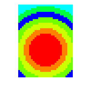
Fig. 3.73 Pseudocolor plot mapping materials to values.