9.1. Annotations

Annotations are objects in the visualization window that convey information about the plots. Annotations can be global objects that show information such as the database name, or they can be objects like plot legends that are directly tied to plots. Annotations are an essential component of a good visualization because they make it clear what is being visualized and make the visualization appear more polished.

VisIt supports several different annotation types that can be used to enhance visualizations. The first category of annotations includes general annotations like the database name, the user name, and plot legends. These annotations convey a good deal of information about what is being visualized, what values are in the plots, and who created the visualization. The second category of annotations include the plot axes and labels. This group of annotations comes in three groups: 2D, 3D and Array. The attributes for these groups can be set independently. Colors can greatly enhance the look of a visualization so VisIt provides controls to set the colors used for annotations and the visualization window that contains them. The third and final category includes annotation objects that can be added to the visualization window. You can add as many annotation objects as you want to a visualization window. The currently supported annotation objects are: 2D text, 3D text, time slider, 2D line, 3D line, and image annotations.

9.1.1. Annotation Window

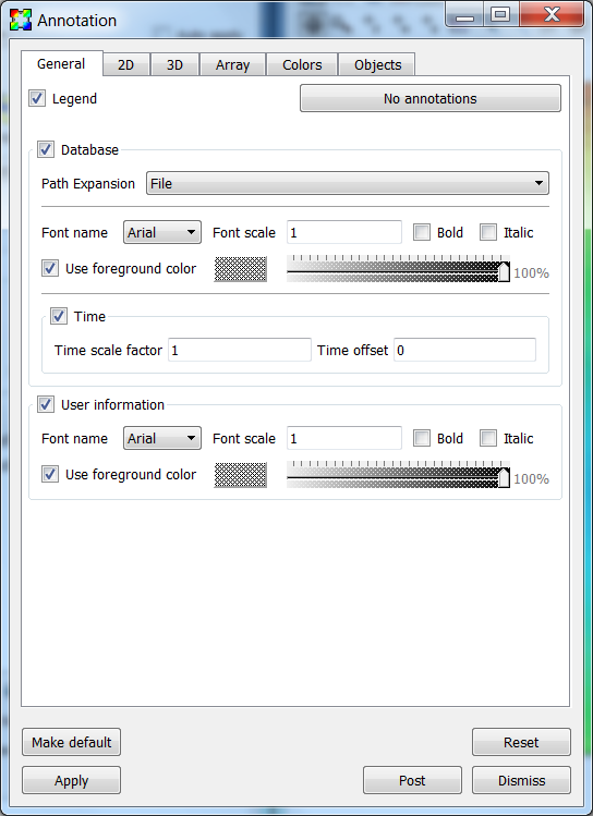
Fig. 9.1 The Annotation window

The Annotation Window (Figure 9.1) contains controls for the various annotations that can appear in a visualization window. You can open the window choosing the Annotation option from the Main Window’s Controls menu. The Annotation Window has a tabbed interface which groups the different categories of annotations together.

9.1.2. General Annotations

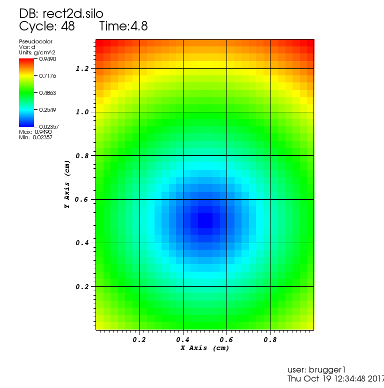
Fig. 9.2 2D plot with annotations

VisIt has a few general annotations that describe the visualization and are independent of the type of database in the visualization. General annotations encompass the user name, the database name, and plot legends. The general annotation controls are located in the General tab. Figure 9.2 shows common locations for some general annotations.

9.1.2.1. Turning plot legends off globally

Plot legends are special annotations that are added by plots. An example of a plot legend is the color bar and title that the Pseudocolor plot adds to the visualization window. Normally, plot legends are turned on or off by a check box in a plot attribute window but VisIt also provides a check box in the General tab that can turn off the plot legends for all the plots in the visualization window. You can use the Legend check box at the top of the General tab to turn plot legends off if they are present.

9.1.2.2. Displaying database information

When plots are displayed in the visualization window, the name of the database used in the plots is shown in the visualization window’s upper left corner. You can turn the database information on or off using the Database check box in the General tab.

The Path Expansion selection box controls the display of the filename text. File causes just the name of the file to be displayed. Directory causes the directory name of the file to be displayed. Full causes the full path of the file to be displayed. Smart uses simulation code specific conventions to display the file name in an optimal fashion. Smart Directory uses simulation code specific conventions to display the directory name in an optimal fashion.

The Time check box controls the display of the time associated with the current database. If Time is enabled then the Time scale factor and Time offset controls become active, allowing you to scale as well as apply an offset to the time associated with a database when displaying it.

9.1.2.3. Displaying user information

When you add plots to the visualization window, your username is shown in the lower right corner. The user information annotation is turned on or off using the User information check box. You may want to turn off user information when you are generating images for presentations.

9.1.3. 2D Annotations

VisIt has a number of controls in the Annotation Window to control 2D annotations on the 2D tab (Figure 9.3). The 2D annotation settings are primarily concerned with the appearance of the 2D axes that frame plots of 2D databases. Figure 9.2 shows a plot with various annotations.

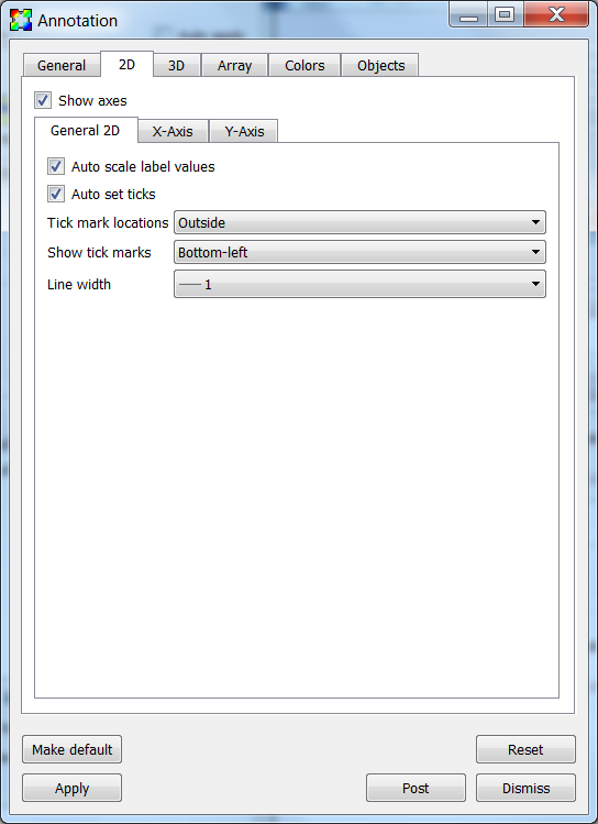
Fig. 9.3 The general 2D properties

The Show axes check box turns on and off the display of the 2D axes.

9.1.3.1. General 2D axis properties

Auto scale label values causes the labels to be multiplied by a factor of 10 to a multiple of 3 power such that the labels are in the range 0.001 to 999. It then displays the multiplier in the axis title. An example is shown in Figure 9.4. The X-Axis range is 0 to 100,000, which causes the labels to be in the range 0 to 100, with a (x10^3) added to the X-Axis and Y-Axis labels to indicate that the true range is actually 0 to 100x10^3 or 100,000.

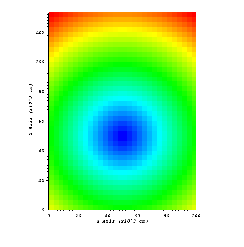
Fig. 9.4 2D plot with axes labels being scaled by 10^3

The tick marks are small lines that are drawn along the edges of the 2D viewport. Tick marks can be drawn on a variety of axes by selecting a new option from the Show tick marks menu. Tick marks can also be drawn on the inside, outside, or both sides of the plot viewport by selecting a new option from the Tick mark locations menu.

Tick mark spacing is usually changed to best suite the plots in the visualization window but you can explicitly set the tick mark spacing by first unchecking the Auto set ticks check box and then typing new tick spacing values into the Major minimum, Major maximum, Major spacing, and Minor spacing text fields in the X-Axis and Y-Axis tabs.

9.1.3.2. Setting the X-Axis and Y-Axis properties

There are tabs for separately controlling the properties of the X and Y axes. The tab for setting the X-Axis properties is shown in Figure 9.5.

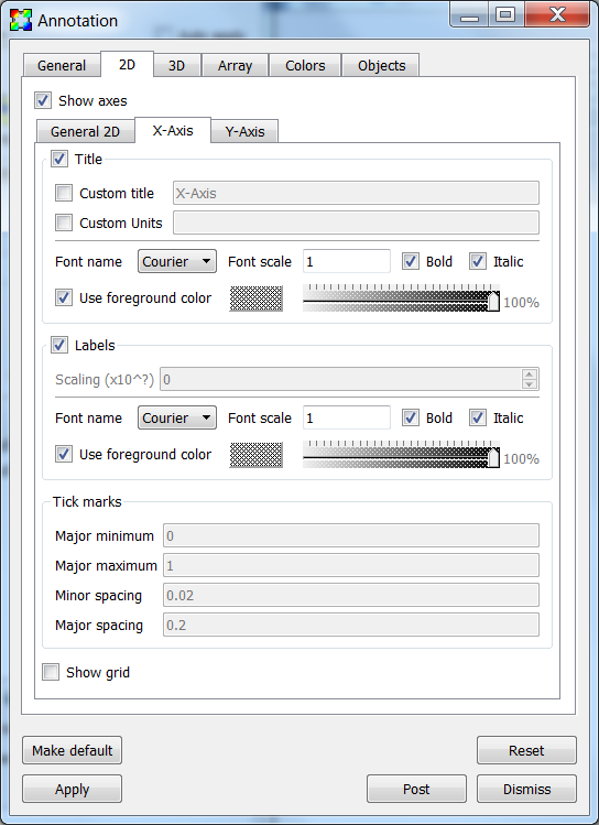
Fig. 9.5 The 2D axes properties

The axis titles are the names that are drawn along each axis, indicating the meaning of the values shown along the axis. Normally, the names used for the axis titles come from the database being plotted so the axis titles are relevant for the displayed plots. Many of VisIt’s database readers plugins read file formats that have no support for storing axis titles so VisIt uses default values such as: “X-Axis”, “Y-Axis”. VisIt provides options that allow you to override the defaults or the axis titles that come from the file. You can control the display of the axis titles by enabling and disabling the Title check box. If you want to override the axis titles that VisIt uses for 2D visualizations, turn on the Custom title check box and type the new axis title into the adjacent text field.

In addition to overriding the names of the axis titles, you can also override the units that are displayed next to the axis titles. Units are displayed only when they are available in the file format and like axis titles, they are not always stored in the file being plotted. If you want to specify units for the axes, turn on the Custom Units check box and type new units into the adjacent text field.

The axis labels are the labels that appear along the 2D plot viewport. By default, the axis labels are enabled and set to appear. You can turn the labels off by unchecking the Labels check box. You can change the label scale factor by changing the Scaling (x10^?) text field.

Tick mark spacing is usually changed to best suite the plots in the visualization window but you can explicitly set the tick mark spacing by first unchecking the Auto set ticks check box on the General 2D tab and then typing new tick spacing values into the Major minimum, Major maximum, Major spacing, and Minor spacing text fields.

The 2D grid lines are a set of lines that make a grid over the 2D viewport. The grid lines are disabled by default but you can enable them by checking the Show grid check box. The grid lines correspond to the major tick marks.

9.1.4. 3D Annotations

VisIt has a number of controls, located on the 3D tab in the Annotation Window for controlling annotations that are used when the visualization window contains 3D plots. Like the 2D controls, these controls focus mainly on the axes that are drawn around plots. Figure 9.6 shows an example 3D plot with the 3D annotations. Figure 9.7 and Figure 9.8 shows the Annotation Window’s 3D tab.

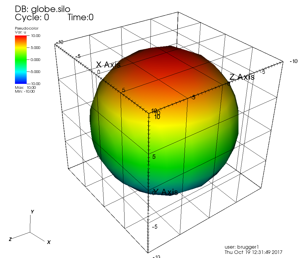
Fig. 9.6 3D plot with annotations

Fig. 9.7 The general 3D properties

The Show axes check box turns on and off the display of the 3D axes.

The Show triad check box turns on and off the display of the triad annotation. The triad annotation consists of a small set of axes and is displayed in the lower left corner of the visualization window and help you get your bearings in 3D.

The Show bounding box check box turns on an off the display of the bounding box. The bounding box annotation displays the edges of a box that contains all the data.

9.1.4.1. General 3D axis properties

Auto scale label values causes the labels to be multiplied by a factor of 10 to a multiple of 3 power such that the labels are in the range 0.001 to 999. It then displays the multiplier in the axis title. A 2D example is shown in Figure 9.4. The X-Axis range is 0 to 100,000, which causes the labels to be in the range 0 to 100, with a (x10^3) added to the X-Axis and Y-Axis labels to indicate that the true range is actually 0 to 100x10^3 or 100,000.

The tick marks are small lines that are drawn along the edges of the bounding box surfaces. Tick marks can be drawn on a variety of axes by selecting a new option from the Show tick marks menu. Tick marks can also be drawn on the inside, outside, or both sides of the plot bounding box by selecting a new option from the Tick mark locations menu.

Tick mark spacing is usually changed to best suite the plots in the visualization window but you can explicitly set the tick mark spacing by first unchecking the Auto set ticks check box and then typing new tick spacing values into the Major minimum, Major maximum, Major spacing, and Minor spacing text fields in the X-Axis, Y-Axis and Z-Axis tabs.

9.1.4.2. Setting the X-Axis, Y-Axis and Z-Axis properties

There are tabs for separately controlling the properties of the X, Y and Z axes. The tab for setting the X-Axis properties is shown in Figure 9.8.

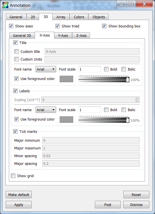
Fig. 9.8 The 3D axes properties

The axis titles are the names that are drawn along each axis, indicating the meaning of the values shown along the axis. Normally, the names used for the axis titles come from the database being plotted so the axis titles are relevant for the displayed plots. Many of VisIt’s database readers plugins read file formats that have no support for storing axis titles so VisIt uses default values such as: “X-Axis”, “Y-Axis” and “Z-Axis”. VisIt provides options that allow you to override the defaults or the axis titles that come from the file. You can control the display of the axis titles by enabling and disabling the Title check box. If you want to override the axis titles that VisIt uses for 3D visualizations, turn on the Custom title check box and type the new axis title into the adjacent text field.

In addition to overriding the names of the axis titles, you can also override the units that are displayed next to the axis titles. Units are displayed only when they are available in the file format and like axis titles, they are not always stored in the file being plotted. If you want to specify units for the axes, turn on the Custom Units check box and type new units into the adjacent text field.

The axis labels are the labels that appear along the edges of the bounding box. By default, the axis labels are enabled and set to appear. You can turn the labels off by unchecking the Labels check box. You can change the label scale factor by changing the Scaling (x10^?) text field.

Tick mark spacing is usually changed to best suite the plots in the visualization window but you can explicitly set the tick mark spacing by first unchecking the Auto set ticks check box on the General 3D tab then typing new tick spacing values into the Major minimum, Major maximum, Major spacing, and Minor spacing text fields.

The 3D grid lines are a set of lines that make a grid over the the bounding box. The grid lines are disabled by default but you can enable them by checking the Show grid check box. The grid lines correspond to the major tick marks.

9.1.5. Annotation Colors

Colors are very important in a visualization since they help to determine how easy it is to read annotations. VisIt provides a tab in the Annotation Window, shown in Figure 9.9, specifically devoted to choosing annotation colors. The Colors tab contains controls to set the background and foreground for the visualization window which, in turn, set the colors used for annotations. The Colors tab also provides controls for more advanced background colors called gradients which are colors that bleed into each other.

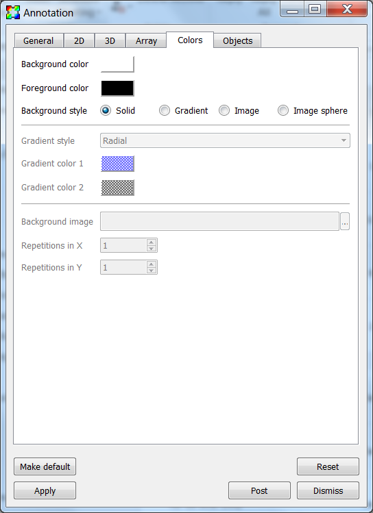
Fig. 9.9 The annotation colors tab

The Background color and Foreground color buttons allow you to set the background and foreground colors. To set the color, click the color button and select a color from the Popup color menu (see Figure 9.10). Releasing the mouse outside of the Popup color menu cancels color selection and the color is not changed. Once you select a new color and click the Apply button, the colors for the active visualization window change. Note that each visualization window can have different background and foreground colors.

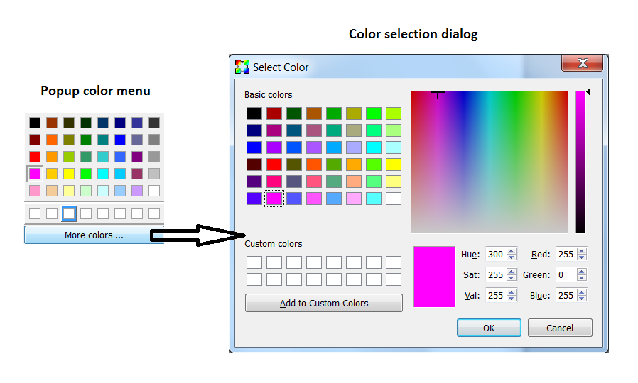
Fig. 9.10 The popup color menu and the color selection dialog

The Background style setting allows you to select from four background styles. The default background style is Solid where the entire background is a single color. The second style is a Gradient background. In a gradient background, two colors are blended into each other in various ways. The resulting background offers differing degrees of contrast and can enhance the look of many visualizations. The third style is an Image background, where an image is tiled across the background. The fourth style is an Image sphere, where an image is projected onto a sphere. This can be used to paint the stars onto the background of an astrophysics simulation. To change the background style, click the Background style radio buttons.

VisIt provides controls for setting the colors and style used for gradient backgrounds. There are two color buttons: Gradient color 1 and Gradient color 2 that are used to change colors. To change the gradient colors, click on the color buttons and select a color from the Popup color menu. The gradient style is used to determine how colors blend into each other. To change the gradient style, make a selection from the Gradient style menu. The available options are Bottom to Top, Top to Bottom, Left to Right, Right to Left, and Radial. The first four options blend gradient color 1 to gradient color 2 in the manner prescribed by the style name. For example, Bottom to Top will have gradient color 1 at the bottom and gradient color 2 at the top. The radial gradient style puts gradient color 1 in the middle of the visualization window and blends gradient color 2 radially outward from the center. Examples of the gradient styles are shown in Figure 9.11.

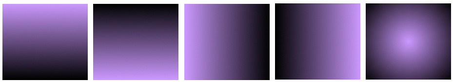
Fig. 9.11 The various gradient styles

The Background image text field allows you to specify the name of the file to use for the background image. The Repetitions in X and Repetitions in Y settings allow you to specify how many times to replicate the image in each of the X and Y image directions.

9.1.6. Annotation Objects

So far, the annotations that have been described can only have a single instance. To provide more flexibility in the types and numbers of annotations, VisIt allows you to create annotation objects, which are objects that are added to the visualization window to convey information about the visualization. Currently, VisIt supports six types of user-creatable annotation objects (2D text, 3D text, time slider, 2D line, 3D line, image) and one automatically generated object tied to specific plots: Legend. All of those types of annotation objects will be described herein. The Objects tab, in the Annotation Window (Figure 9.12 ) is devoted to managing the list of annotation objects and setting their properties.

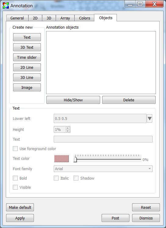
Fig. 9.12 The annotation objects tab

The Objects tab in the Annotation Window is divided up into three main areas. The top of the window is split vertically into two areas that let you create new annotation objects and manage the list of annotation objects. The bottom half of the Objects tab displays the controls for setting the attributes of the selected annotation object. Each annotation object provides a separate user interface that is tailored for setting its particular attributes. When you select an annotation in the annotation object list, the appropriate annotation object interface is displayed.

9.1.6.1. Creating a new annotation object

The Create new area in the Annotation Window’s Objects tab contains one button for each type of annotation object that VisIt can create. Each button has the name of the type of annotation object VisIt creates when you push it. After pushing one of the buttons, VisIt creates a new instance of the specified annotation object type, adds a new entry to the Annotation objects list, and displays the appropriate annotation object interface in the bottom half of the Objects tab to display the attributes for the new annotation object.

9.1.6.2. Selecting an annotation object

The Objects tab displays the annotation object interface for the selected annotation object. To set attributes for a different annotation object, or to hide or delete a different annotation object, you must first select a different annotation object in the Annotation objects list. Click on a different entry in the Annotation objects list to highlight a different annotation object. Once you have highlighted a new annotation object, VisIt displays the object’s attributes in the lower half of the Objects tab.

9.1.6.3. Hiding an annotation object

To hide an annotation object, select it in the Annotation objects list and then click the Hide/Show button on the Objects tab. To show the hidden annotation object, click the Hide/Show button a second time. The interfaces for the currently provided annotation objects also have a Visible check box that can be used to hide or show the annotation object.

9.1.6.4. Deleting an annotation object

To delete an annotation object, select it in the Annotation objects list and then click the Delete button on the Objects tab. You can delete more than one object if you select multiple objects plots in the Annotation objects list before clicking the Delete button.

9.1.6.5. Text annotation objects

Text annotation objects, shown in Figure 9.13, are created by clicking the Text button in the Create new area on the Objects tab. Text annotation objects are simple 2D text objects that are drawn on top of plots in the visualization window and are useful for adding titles to a visualization.

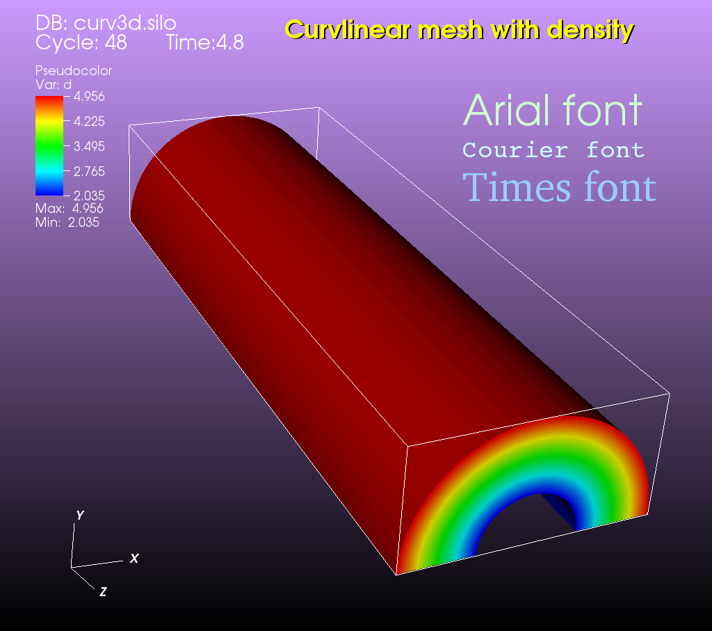
Fig. 9.13 Examples of text annotations

The text annotation object properties, shown in Figure 9.14, can be used to set the position, size, text, colors, and font properties.

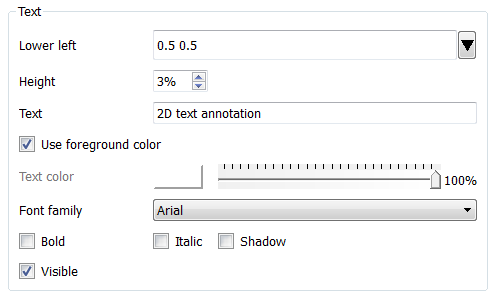
Fig. 9.14 The text annotation interface

Text annotation objects are placed using 2D coordinates where the X, and Y values are in the range [0,1]. The point (0,0) corresponds to the lower left corner of the visualization window and the point (1,1) corresponds to the upper right of the visualization window. The 2D coordinate used to position the text annotation matches the text annotation’s lower left corner. To position a text annotation object, enter a new 2D coordinate into the Lower left text field. You can also click the down arrow next to the Lower left text field to interactively choose a new lower left coordinate for the text annotation using the screen positioning control, which represents the visualization window. The screen positioning control, shown in Figure 9.15, lets you move a set of cross-hairs to any point on a square area that represents the visualization window. Once you release the left mouse button, the location of the cross-hairs is used as the new coordinate for the text annotation object’s lower left corner.

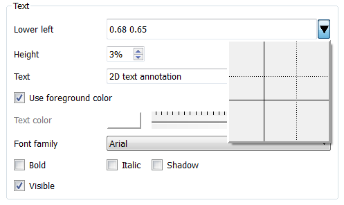
Fig. 9.15 Screen positioning control

The size of the text is set using the Height spin box. The height is the fraction of the visualization window height.

To set the text that a text annotation object displays, type a new string into the Text text field. You can make the text annotation object display any characters that you type in. Whatever text you enter for the text annotation object is used to identify the text annotation object in the Annotation objects list. In addition to the usual text properties, text annotation objects can also include a shadow.

9.1.6.6. Named database values in text annotations

A variety of named database values can be displayed in text annotations. These are introduced with a leading $ character followed by the value’s name. An optional % character following the value’s name introduces a printf-style formatting string which can be used to control the value’s printed format.

Warning

Presently, the $ values that are displayed are taken always from database associated with the first plot in the plot list. If the plot list is changed such that the database associated with the first plot that was in effect at the time the annotation was created is changed, the rendered text for named database value annotations may change.

The list of named values currently supported along with their default formats are

Value name	Fmt	Meaning
time	%g	time value
cycle	%d	cycle number
index	%d	state number starting from zero
numstates	%d	total number of states in database
dbcomment	%s	database comment
lod	%z	levels of detail
vardim	%d	variable dimension
numvar	%d	number of variables
topdim	%d	topological dim. of assoc. mesh
spatialdim	%d	spatial dim. of assoc. mesh
varname	%s	variable name
varunits	%s	variable units
meshname	%s	name of mesh assoc. w/variable
filename	%s	name of database file
fulldbname	%s	full path name of database file
xunits	%s	x units
yunits	%s	y units
zunits	%s	z units
xlabel	%s	x axis label
ylabel	%s	y axis label
zlabel	%s	z axis label

In addition, the following $<T>tafile<I> named values permit arbitrary text annotation content to be taken from a txt file with name of the form <T>tafile<I>.txt where <T> is either s (for files of string values), i (for files of integer values) or f (for files of floating point values) and <I> is either 1, 2 or 3 to provide 3 separate options for storing files of values used for different annotation purposes. Each line of such a file corresponds to a time step in a time series. If a $$<T>tafile<I> named annotation is used, VisIt will search for the associated file first in the same directory containing the database, then in the directory /$TMPDIR/$USER or (/var/tmp/$USER) and finally in The Platform and the User’s Home Directory.

A common use case for $<T>tafile<I> named values is for animations to display the numerical values from a query over time and have those values update as the time step being displayed changes.

Value name	Fmt	Meaning
itafile1	%d	ints from itafile1.txt one line per timestep.
itafile2	%d	ints from itafile2.txt one line per timestep.
itafile3	%d	ints from itafile3.txt one line per timestep.
ftafile1	%g	floats from ftafile1.txt one line per timestep.
ftafile2	%g	floats from ftafile2.txt one line per timestep.
ftafile3	%g	floats from ftafile3.txt one line per timestep.
stafile1	%s	strings from stafile1.txt one line per timestep.
stafile2	%s	strings from stafile2.txt one line per timestep.
stafile3	%s	strings from stafile3.txt one line per timestep.

Warning

Only the first 255 characters on each line of a $<T>tafile<I> annotation are used.

Multiple named values can appear in a text annotation string and the same named value can also appear multiple times.

For example, to create a text annoation which displays State index = XXX where XXX is the number for the index, set the annotation string to State index = $index. To display the current cycle number always with 6 digits and leading zeros when necessary, use the string $cycle%06d where the optional % followed by a printf-style format string is specified. To display the first 3 characters of the variable name, use the string $varname%.3s.

The $dbcomment and $<T>tafile<I> named values are useful for complicated cases because they allow arbitrary text defined in the database comment or an external file to be used. For example, the state space of a given database could be rather complicated involving not only iterations of the main PDE solve loop but also mesh adaptivity iterations, material advection iterations, etc. In this case, if the data producer created appropriate content in the database comment or in a text file, the $dbcomment or $<T>tafile<X> named value is a way to render all relevant iteration identifiers as a text annotation.

9.1.6.7. 3D text annotation objects

3D text annotation objects, shown in Figure 9.16, are created by clicking the 3D Text button in the Create new area on the Objects tab. 3D text annotation objects are extruded text that are positioned in 3D and are part of the 3D scene, so they may become obscured by other objects in the scene and will move in space as the image is panned and zoomed.

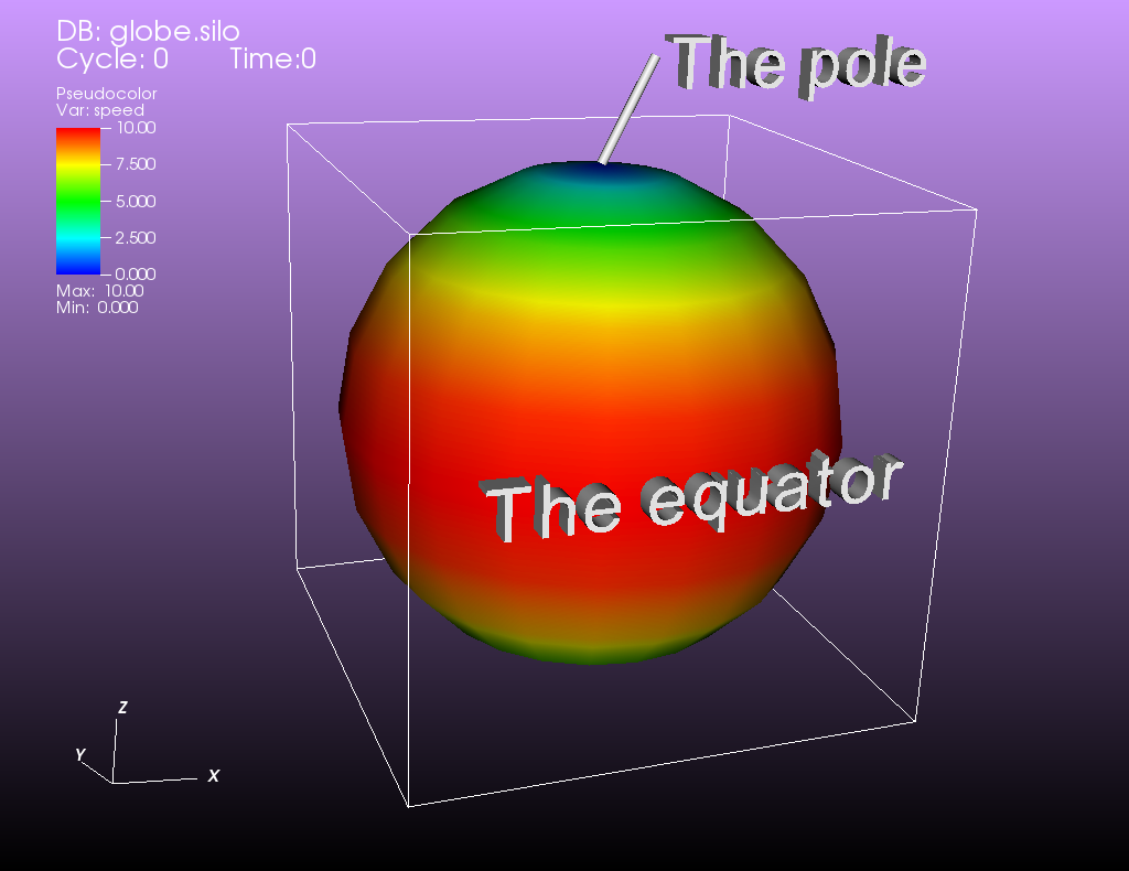
Fig. 9.16 Examples of 3d text annotations

The 3D text annotation object properties, shown in Figure 9.17, can be used to set the text, position, size, orientation and color properties.

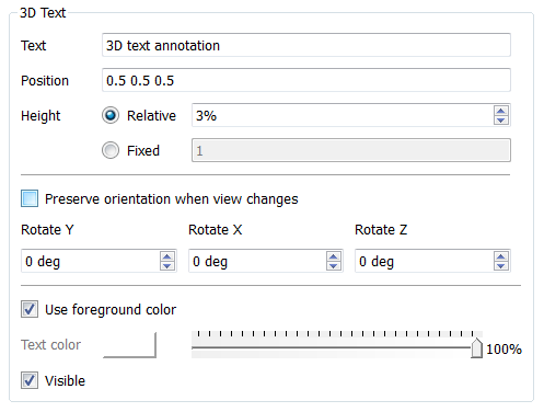
Fig. 9.17 The 3D text annotation interface

To set the text that a 3D text annotation object displays, type a new string into the Text text field.

3D text annotation objects are placed in 3D coordinates in the same coordinate system used by the simulation data. To position a 3D text annotation object, enter a new 3D coordinate into the Position text field.

The size of the text can be specified in two different ways. The first is using a relative height, where the height is a fraction of the size of the simulation data. The second is a fixed size, where the size is specified in the coordinate system of the simulation data. If you were to specify a relative height and apply the Transform operator to scale the data in each direction by a factor of 10, the size of the text would not change. If you were to specify a fixed height, scaling the data by a factor of 10 would result in the text being one tenth the size. To specify a relative height, select the Relative radio button and set the size using the spin box next to it. The specify a fixed height, select the Fixed radio button and enter the new height in the text box next to it.

The orientation of the text can also be specified in two different ways. The first is relative to the screen coordinate system and the second is in the coordinate system of the simulation data. If the orientation is relative to the screen coordinate system, then rotating the image will not change the orientation of the text. If the orientation is relative to the coordinate system of the simulation data, then rotating the image will change the orientation of the text. To make the orientation relative to the screen, select the Preserve orientation when view changes radio button. To make the orientation relative to the simulation coordinate system, uncheck the Preserve orientation when view changes radio button. To set the orientation, set the Rotate Y, Rotate X and Rotate Z spin boxes. The rotations are applied in the left to right order of the spin boxes in the interface.

9.1.6.8. Time slider annotation objects

Time slider annotation objects, shown in Figure 9.18, are created by clicking the Time slider button in the Create new area on the Objects tab. Time slider annotation objects consist of a graphic that shows the progress through an animation using animation and text that shows the current database time. Time slider annotation objects can be placed anywhere in the visualization window and you can set their size, text, colors, and appearance properties.

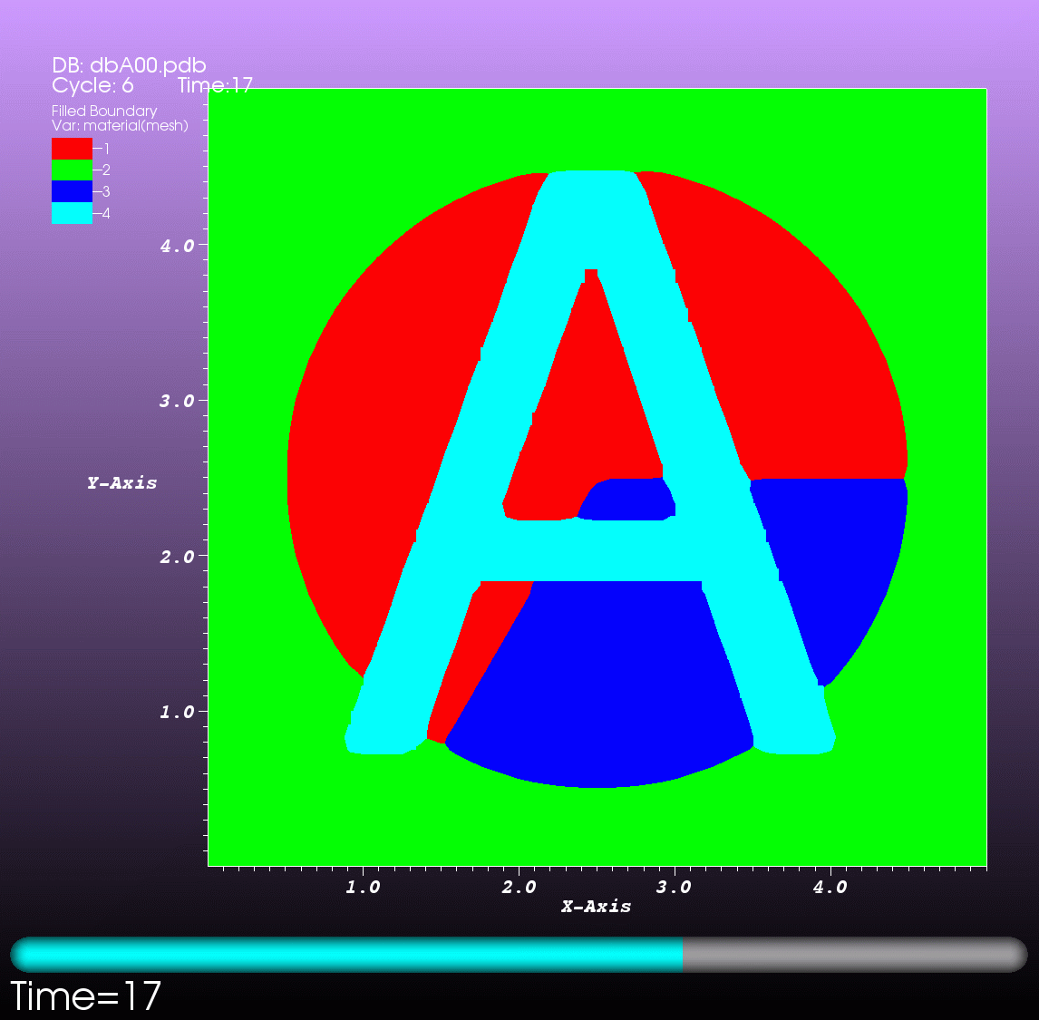
Fig. 9.18 An example of a time slider annotation object

Time slider annotation objects are placed using 2D coordinates where the X, and Y values are in the range [0,1]. The point (0,0) corresponds to the lower left corner of the visualization window and the point (1,1) corresponds to the upper right of the visualization window. The 2D coordinate used to position the text annotation matches the text annotation’s lower left corner. To position a text annotation object, enter a new 2D coordinate into the Lower left text field. You can also click the down arrow next to the Lower left text field to interactively choose a new lower left coordinate for the text annotation using the screen positioning control, which represents the visualization window.

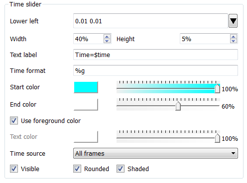
Fig. 9.19 The time slider interface

The size of a time slider annotation object is controlled by settings its height and width as a percentage of the visualization window height and width. Type new values into the Width and Height spin buttons to set a new width or height for the time slider annotation object.

You can set the text displayed by the time slider annotation object by typing a new text string into the Text label text field. Text is displayed below the time slider annotation object and it can contain any message that you want. The text can even include wildcards such as $time, which evaluates to the current time for the active database. If you use $time to make VisIt incorporate the time for the active database, you can also specify the format string used to display the time. The format string is a standard C-language format string (e.g. “%4.6g”) and it determines the precision used to write out the numbers used in the time string. You will probably want to specify a format string that uses a fixed number of decimal places to ensure that the time string remains the same length during the animation, preventing distracting differences in the length of the string from taking the eye away from the visualization. Type a C-language format string into the Time format text field to change the time format string.

Time slider annotations have three color attributes: start color, end color, and text color. A time slider annotation object displays time like a progress bar in that the progress bar starts out small and then grows to the right until it takes up the whole length of the annotation. The color used to represent the progress can be set by clicking the Start color button and choosing a new color from the Popup color menu. As the time slider annotation object shows more progress, the color that is used to fill up the time that has not been reached yet (end color) is overtaken by the start color. To set the end color for the time slider annotation object, click the End color button and choose a new color from the Popup color menu. Normally, time slider annotation objects use the foreground color of the visualization window when drawing the annotation’s text. If you want to make the annotation use a special color, turn off the Use foreground color check box and click the Text color button and choose a new color from the Popup color menu.

Time slider objects have two more attributes that affect their appearance. The first of those attributes is set by clicking on the Rounded check box. When a time slider annotation object is rounded, the ends of the annotation are curved. The last attribute is set by clicking on the Shaded check box. When a time slider annotation object is shaded, simple lighting is applied to its geometry and the annotation will appear to be more 3-dimensional.

9.1.6.9. 2D line annotation objects

2D line annotation objects, shown in Figure 9.21, are created by clicking the 2D Line button in the Create new area on the Objects tab. 2D line annotation objects are simple line objects that are drawn on top of plots in the visualization window and are useful for pointing to features of interest in a visualization. 2D line annotation objects can be placed anywhere in the visualization window and you can set their locations, arrow properties, and color.

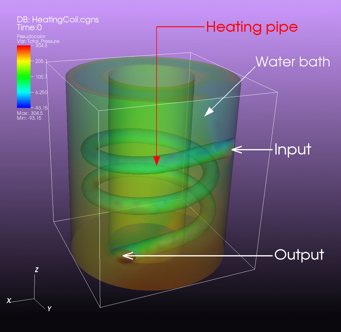
Fig. 9.20 Examples of 2D line annotations

2D line annotations are described mainly by two coordinates that specify the start and end points for the line. The start and end coordinates are specified as pairs of floating point numbers in the range [0,1] where the point (0,0) corresponds to the lower left corner of the visualization window and the point (1,1) corresponds to the upper right corner of the visualization window. You can set the start or end points for the 2D line annotation by entering new start or end points into the Start or End text fields in the 2D line object interface. You can also click the down arrow to the right of the Start or End text fields to interactively choose new coordinates using the screen positioning control.

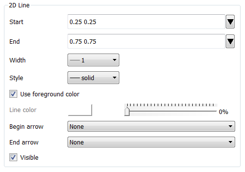
Fig. 9.21 The 2D line object interface

Once the 2D line annotation has been positioned there are other attributes that can be set to improve its appearance. First of all, if the 2D line annotation is being used to point at important features in a visualization, you might want to increase the 2D line annotation’s width to make it stand out more. To change the width, select the new pixel width from the Width menu. It is also possible to set the line style. To change the style of the line, select the new line style from the Style menu. After changing the width and style, the color of the 2D line annotation should be chosen to stand out against the plots in the visualization. The color that you use should be chosen such that the line contrasts sharply with the plots over which it is drawn. To choose a new color for the line, click on the Line color button and choose a new color from the Popup color menu. You can also adjust the opacity of the line by using the opacity slider next to the Line color button.

The last properties that are commonly set for 2D line annotations determine whether the end points of the line have arrow heads. The 2D line annotation supports two different styles of arrow heads: filled and lines. To make your line have arrow heads at the start or the end, make new selections from the Begin arrow and End arrow menus.

9.1.6.10. 3D line annotation objects

3D line annotation objects, shown in Figure 9.16, are created by clicking the 3D Line button in the Create new area on the Objects tab. 3D line annotation objects are lines that are positioned in 3D and are part of the 3D scene, so they may become obscured by other objects in the scene and will move in space as the image is panned and zoomed.

The 3D line annotation object properties, shown in Figure 9.22, can be used to set the position, style and color properties.

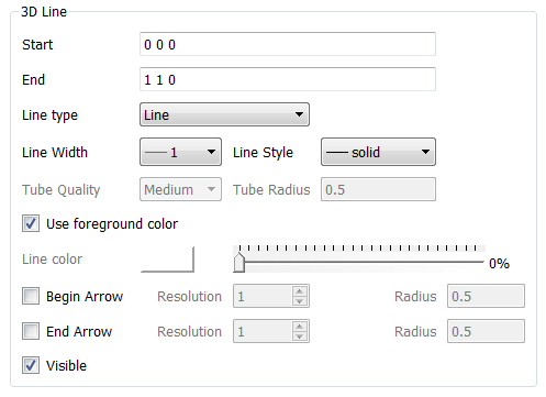
Fig. 9.22 The 3D line object interface

3D text annotation objects are placed in 3D coordinates in the same coordinate system used by the simulation data. To position a 3D line annotation object, specify the start and end location of the line by entering the start location in the Start text field and the end location in the End text field.

There are two types of lines supported, one is a normal line and the other is a tube. The line type is selected through the Line type menu. When using a normal line, you can specify the normal line width and line style properties using the Line Width and Line Style menus. When using a tube you can specify the tube quality and radius. The tube is created from a series of flat surfaces around the center of the line to approximate a tube. The number of surfaces used is controlled by the tube quality. The tube radius is the radius of the tube in the coordinate system of the simulation data. These properties can be changed through the Tube Quality and Tube Radius menus.

It is also possible to add arrows to the beginning and end of the line. These can be enabled with the Begin Arrow and End Arrow toggle buttons. For each arrow, the user can also control the resolution and radius of the arrows. The arrows consist of cones places at the ends of the line and are constructed out of triangles that approximate a cone. The number of triangles used is controlled by the resolution. The radius is the radius of the cone in the same coordinate system as the simulation data. The resolution can be changed using the Resolution spin box and the radius is changed by typing a new value into the Radius text field.

9.1.6.11. Image annotation objects

Image annotation objects, shown in Figure 9.23, are created by clicking the Image button in the Create new area on the Objects tab. Image annotation objects display images from image files on disk in a visualization window. Images are drawn on top of plots in the visualization window and are useful for adding logos, pictures of experimental data, or other views of the same visualization. Image annotation objects can be placed anywhere in the visualization window and you can set their size, and optional transparency color.

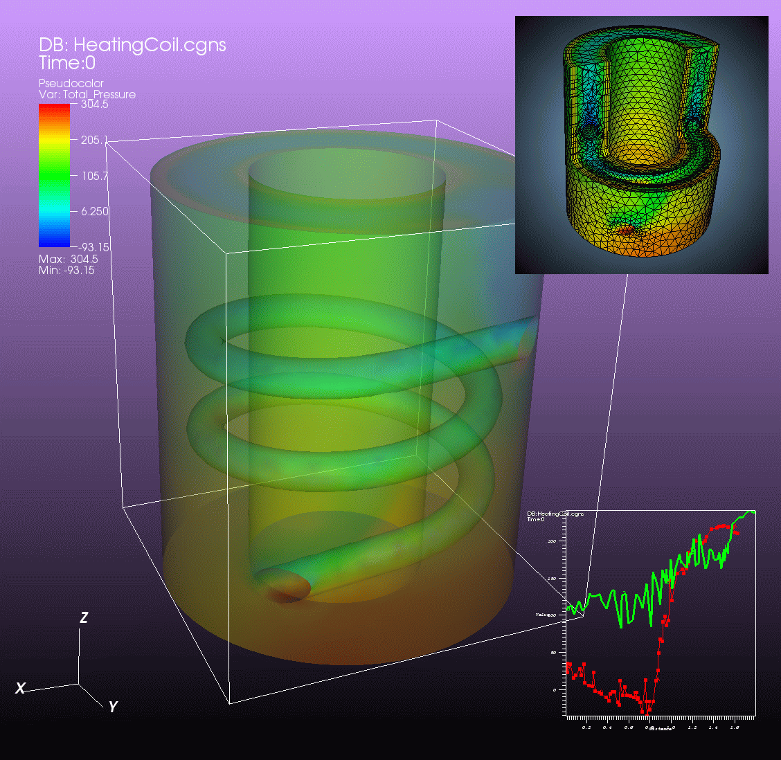
Fig. 9.23 An Example of a visualization with two overlaid image annotations

The first step in incorporating an image annotation into a visualization is to choose the file that contains the image that will serve as the annotation. To choose an image file for the image annotation, type in the full path and filename to the file that you want to use into the Image source text field. You can also use the file browser to locate the image file if you click on the “…” button to the right of the Image source text field in the Image annotation interface, shown in Figure 9.24.

Warning

Currently, there is a limitation in the use of image annotations while operating in client/server mode. The path used must be the same on both the local (client) and remote (server) machines. Often, the only way to achieve this may be to have the image file in /tmp or /var/tmp. For parallel engines, this may necessitate a complicated set of manual steps to a) wait for the parallel job to start, b) identify the node running MPI rank 0 (the only MPI rank where annotations are processed) and c) copy the file to the /tmp directory on that node assuming access controls will even allow that.

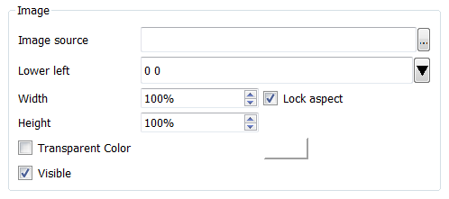
Fig. 9.24 The image object interface

After selecting an image file, you can position its lower left coordinate in the visualization window. The lower left corner of the visualization window is the origin (0,0) and the upper right corner of the visualization window is (1,1).

Once you position the image where you want it, you can optionally scale it relative to its original size. Unlike some other annotation objects, the image annotation does not scale automatically when the visualization window changes size. The image annotation will remain the same size - something to take into account when setting up movies that use the image annotation. To scale the image relative to its original size, enter new percentages into the Width and Height spin boxes. If you want to scale one dimension of the image and let the other dimension remain unchanged, turn off the Lock aspect check box.

Finally, if you are overlaying an image annotation whose image contains a constant background color or other area that you want to remove, you can pick a color that VisIt will make transparent. For example, Figure 9.23 shows an image of some Curve plots overlaid on top of the plots in the visualization window and the original background color in the annotation object was removed to make it transparent. If you want to make a color in an image transparent before VisIt displays it as an image annotation object, click on the Transparent color check box and then select a new color by clicking on the Transparent color button and picking a new color from the Popup color menu.

9.1.6.12. Legend annotation objects

Legends are automatically added when plots are created, and have names that include the plot type. Figure 9.25 shows multiple legends listed in the Annotation Objects tab. The Legend annotation object interface can be used to customize the legends position, size, tick labels and aspects of its appearance.

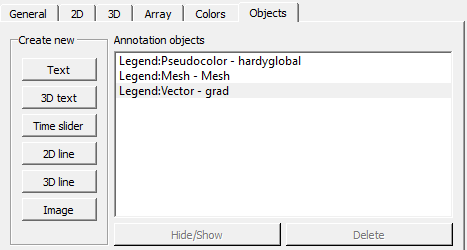
Fig. 9.25 Multiple legends in the Annotation Objects tab.

The Position tab, shown in Figure 9.26 has controls for position, size and orientation. VisIt generally controls the positions of legends, but if you want a specific legend to be placed elsewhere in the visualization window, uncheck the Let VisIt manage legend position checkbox and modify the Legend position. The 2D coordinate used to position the legend matches the legend’s lower left corner. To change the position of a legend, enter a new 2D coordinate into the Legend position text field. You can also click the down arrow next to the Legend position text field to interactively choose a new lower left coordinate using the screen positioning control, which represents the visualization window. The screen positioning control, shown in Figure 9.15, lets you move a set of cross-hairs to any point on a square area that represents the visualization window. Once you release the left mouse button, the location of the cross-hairs is used as the new coordinate for the legend’s lower left corner.

The X scale and Y scale spin boxes control the size of the legend, with values of ‘100%’ being the default size. You can enter new values using the text field or use the + and - buttons to the right of the text field.

The Orientation of the legend is changed using the corresponding drop-down menu, with options: Vertical, Text on Right; Vertical, Text on Left; Horizontal, Text on Top and Horizonatal, Text on Bottom.

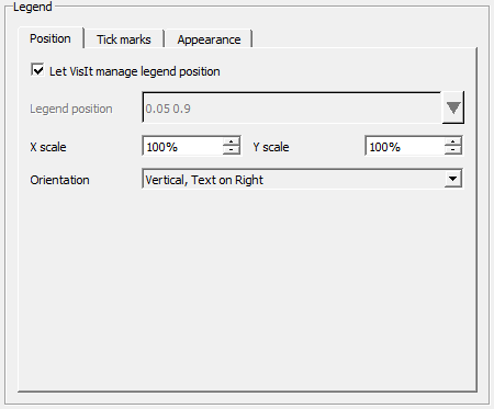
Fig. 9.26 The legend object interface for position

The Tick marks tab, shown in Figure 9.27, allows you to change the display of a legend’s tick marks. You can turn off the drawing of tickmarks completely by choosing the None option in the Draw dropdown menu. Other Draw options are Values (the default), Labels and Values and Labels. Legends usually only have Values defined for tick marks, so to display Labels, you would have to define them by unchecking the Let VisIt determine tick labels checkbox and modifying the Specify tick values and labels table. It starts out with the Values column filled in with defaults. You can modify those, add text to the Labels column and change the number of table items by using the Add tick value and Delete selected value buttons. When modifying, adding, or deleting values in the table, keep in mind they must fall within the Min/Max range of the current plot or they won’t be displayed in the legend. Not all plot types allow adding or deleting values.

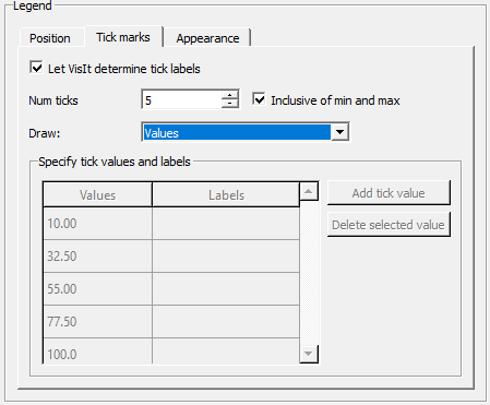
Fig. 9.27 The legend object interface for tick marks

Figure 9.28 shows an example of modifying and displaying Labels for a Boundary and FilledBoundary Plots. The Values have both a number and the name of the material, and the Labels were added so that only the material names would be displayed in the legend.

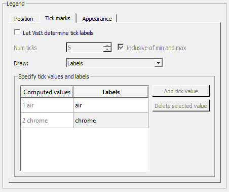
Fig. 9.28 An example of modifying the Labels on a filled boundary legend

Figure 9.29 shows the controls for changing the Appearance of a legend.

The Bounding box checkbox controls whether or not a background bounding box is drawn behind the legend. When checked, widgets for controlling the color and opacity of the background bounding box will become active.

The title can be turned off via the Draw title checkbox. A custom title can be specified via the Custom title checkbox and text edit widgets.

The Draw min/max checkbox controls whether or not Min/Max text (where applicable) will be added to the legend.

By unchecking the Use foreground color checkbox, you can change the color of the legend’s text and tickmarks via the Text color button.

Number format controls the fromat for tick mark and Min/Max values. You can modify the font style via the Font height text edit, Font family dropdown menu and Bold and Italic check boxes. (Shadow is currently disabled).

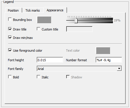
Fig. 9.29 The legend object interface for appearance

Figure 9.30 shows an example of a modified legend, where position, orientation, size, tick marks, background font height and font family have all been changed.

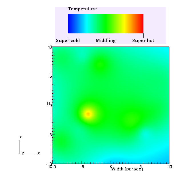
Fig. 9.30 Example of a modified legend