3.2.2. Boundary and FilledBoundary Plots

The Boundary plot and FilledBoundary plot are discussed together because of their similarity. Both plots concentrate on the boundaries between materials but each plot shows the boundary in a different way. The Boundary plot, shown in Figure 3.8, displays the surface or lines that separate materials.

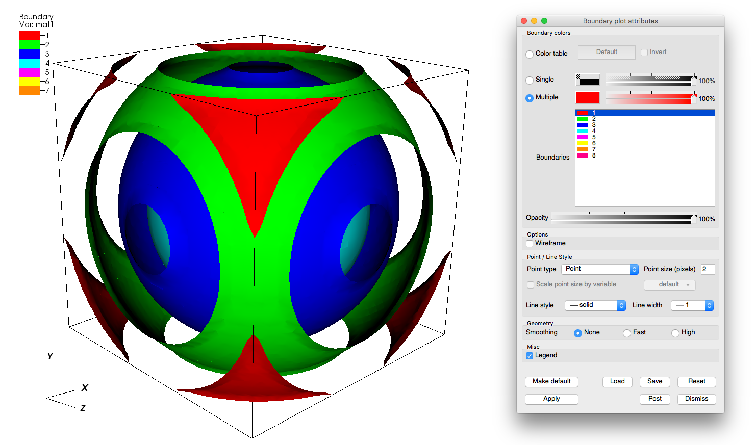
Fig. 3.8 Boundary plot and its plot attributes window

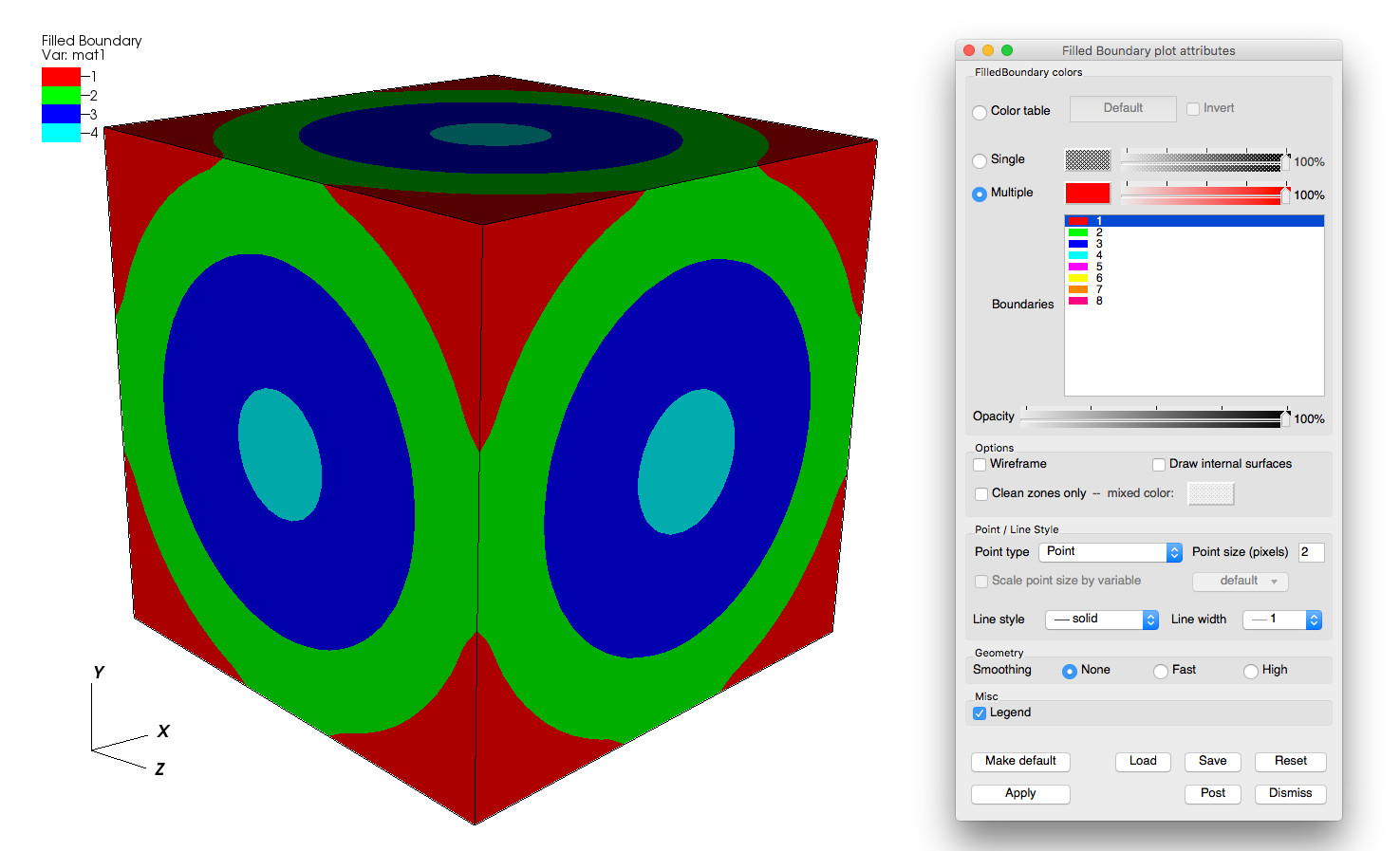
Fig. 3.9 FilledBoundary plot and its plot attributes window

The FilledBoundary plot (see Figure 3.9) shows the entire set of materials, each using a different color. Both plots perform material interface reconstruction on materials that have mixed cells, resulting in the material boundaries used in the plots.

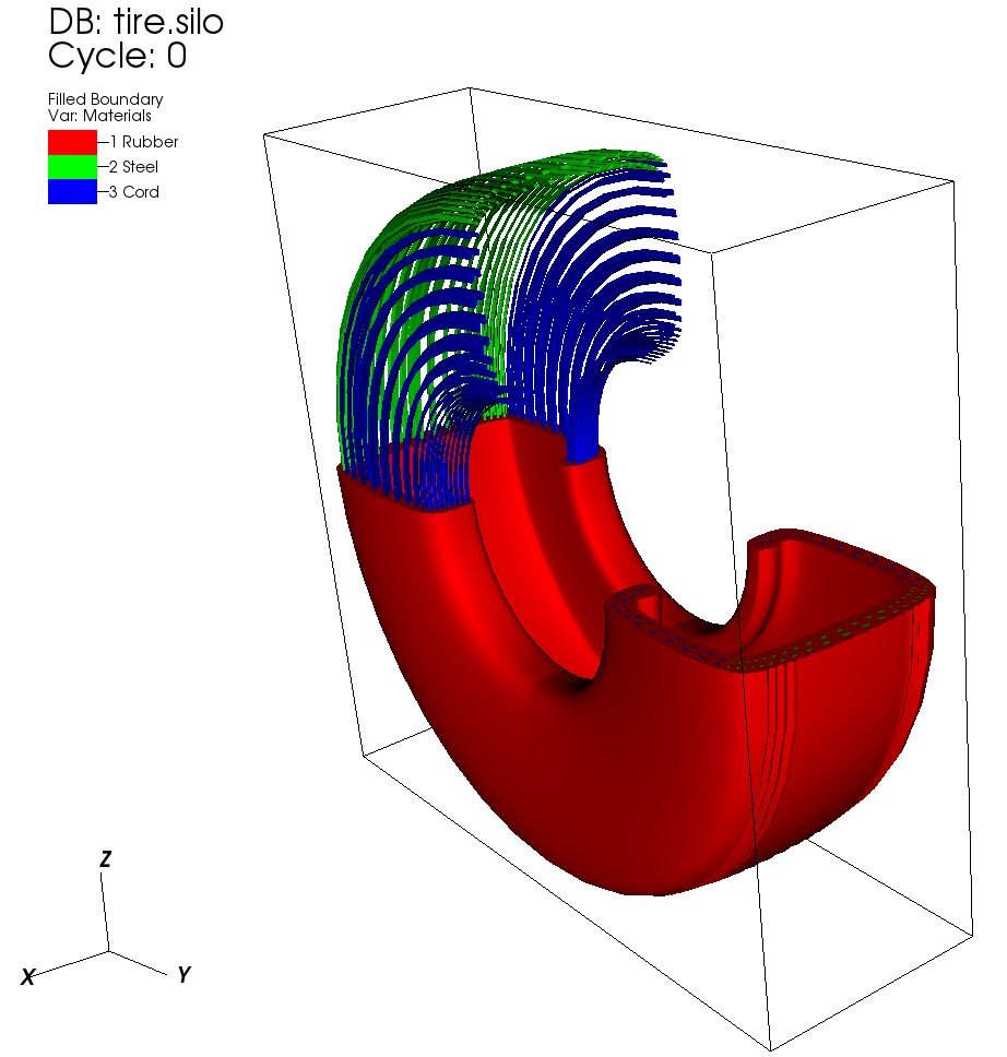
Fig. 3.10 FilledBoundary plot combined with subsets

Combining the FilledBoundary plot with subsets (see Figure 3.10) can provide a insight into where each material is inside the mesh by turning off materials in a particular domain. For more information about subsets, see the Subsetting chapter. .

3.2.2.1. Changing colors

The main portion of the Boundary plot attributes window and FilledBoundary plot attributes window, also known as the Boundary colors area, is devoted to setting material boundary colors. The Boundary colors area contains a list of material names with an associated material color. Boundary plot and FilledBoundary plot colors can be assigned three different ways, the first of which uses a color table. A color table is a named palette of colors that you can customize to suite your needs. When the Boundary plot or FilledBoundary plot use a color table to color subsets, they selects colors that are evenly spaced through the color table based on the number of subsets. For example, if you have three materials and you are coloring them using the “xray” color table, three colors are picked out of the color table so your material boundaries are colored black, gray, and white. To color a Boundary plot or FilledBoundary plot with a color table, click on the Color table radio button and choose a color table from the Color table menu to right of the Color table radio button.

If you want all subsets to be the same color, click the Single radio button at the top of the Boundary plot attributes window and select a new color from the Popup color menu that is activated by clicking on the Single color button. The opacity slider next to the Single color button sets the opacity for the single color.

Clicking the Multiple radio button causes each material boundary to be a different, user-specified color. By default, multiple colors are set using the colors of the discrete color table that is active when the Boundary or FilledBoundary plot is created. To change the color for any of the materials, select one or more materials from the list of materials and click on the Color button to the right of the Multiple radio button and select a new color from the Popup color menu. To change the opacity for a material, move Multiple opacity slider to the left to make the material more transparent or move the slider to the right to make the material more opaque.

The Boundary plot attributes window contains a list of material names with an associated color. To change a material’s color, select one or more materials from the list, click the color button and select a new color from the popup color menu.

3.2.2.2. Opacity

The Boundary plot’s opacity can be changed globally as well as on a per material basis. To change material opacity, first select one or more materials in the list and move the opacity slider next to the color button. Moving the opacity slider to the left makes the selected materials more transparent and moving the slider to the right makes the selected materials more opaque. To change the entire plot’s opacity globally, use the Opacity slider near the bottom of the window.

3.2.2.3. Wireframe mode

The Boundary plot and the FilledBoundary plot can be modified so that they only display outer edges of material boundaries. This option usually leaves lines that give only the rough shape of materials and where they join other materials as seen in. To make the Boundary or FilledBoundary plots display in wireframe mode, check the Wireframe check box near the bottom of the window.

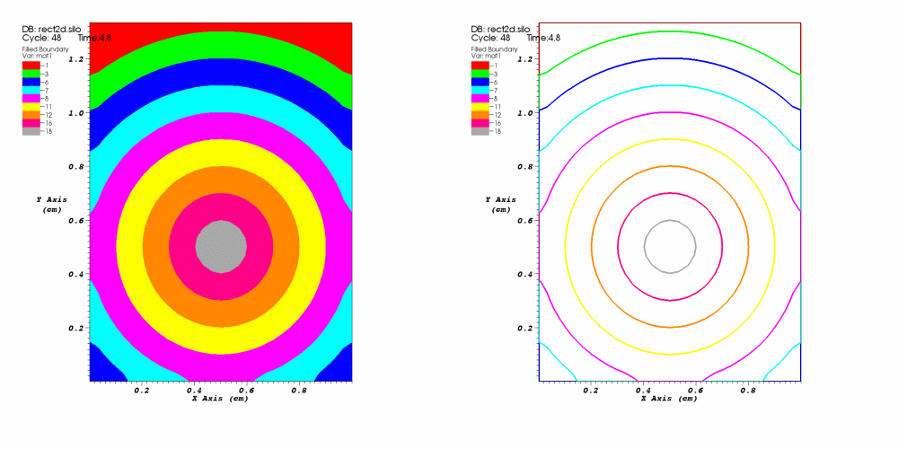
Fig. 3.11 Filled mode and wireframe mode

3.2.2.4. Geometry smoothing

Sometimes visualization operations such as material interface reconstruction can alter mesh surfaces so they are pointy or distorted. The Boundary plot and the FilledBoundary plot provide an optional Geometry smoothing option to smooth out the mesh surfaces so they look better when the plots are visualized. Geometry smoothing is not done by default, you must click the Fast or High radio buttons to enable it. The Fast geometry smoothing setting smooths out the geometry a little while the High setting works produces smoother surfaces.

3.2.2.5. Drawing only clean zones

The FilledBoundary plot, since it deals almost exclusively with plotting materials, has an option to only draw clean zones, which are zones that contain a single material. When only clean zones are drawn, all clean cells are drawn normally but all zones that contained more than one material are drawn with a color that can be set to match the vis window’s background color (see). Drawing clean zones is primarily used to examine how materials mix in 2D databases. To make VisIt draw only the clean zones, click the Clean zones only check box. After that, you can set the mixed color by clicking on the Mixed color color button and selecting a new color from the popup color palette.

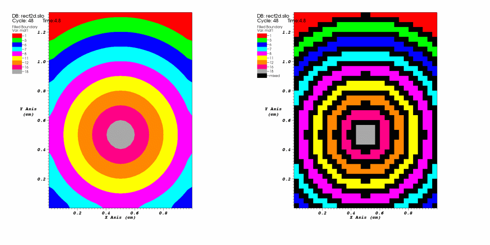
Fig. 3.12 All zones and clean zones

3.2.2.6. Setting point properties

Albeit rare, the Boundary and FilledBoundary plots can be used to plot points that belong to different materials. Both plots provide controls that allow you to set the representation and size of the points. You can change the points’ representation using the different Point Type radio buttons. The available options are:

• Box

• Axis

• Icosahedron

• Octahedron

• Tetrahedron

• Point

• Sphere

The default point type is Point because that is the fastest to draw, followed by Sphere. The other point types create additional geometry and can take longer to appear on the screen and subsequently draw. To change the size of the points when the point type is set to Box, Axis, or Icosahedron, you can enter a new floating point value into the Point size text field. When the point type is set to Point or Sphere, the Point size text field becomes the Point size (pixels) text field and you should enter your point size in terms of pixels. Finally, you can opt to scale the points’ glyphs using a scalar expression by turning on the Scale point size by variable check box and by selecting a scalar variable from the Variable button to the right of that check box. Note that point scaling does not occur when the point type is set to Point or Sphere.

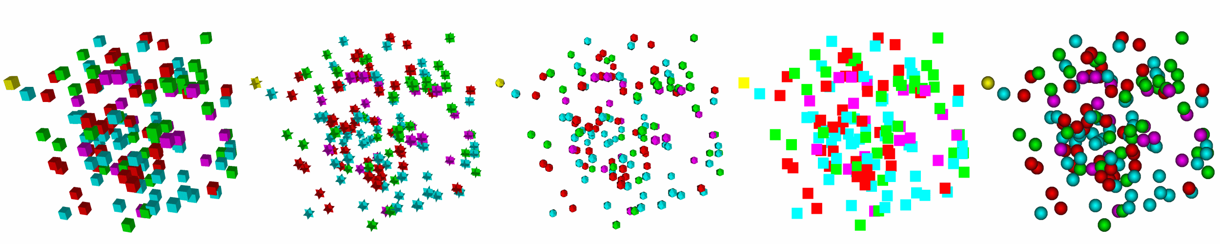
Fig. 3.13 Point types (left-to-right): Box, Axis, Icosahedron, Point, Sphere