7. Connected Components
VisIt provides an expression and set of queries to help identify and summarize connected subcomponents of a mesh. These capabilities can help isolate or compute statistics of complex features embedded in your data. The connected components algorithm used is unique in that it can not only process simple meshes, but it can also efficiently handle large meshes partitioned in a distributed-memory setting. This tutorial provides an introduction of how to use VisIt’s connected components capabilities. The algorithm is not discussed here, for more details on the algorithm see [1] .
7.1. Open the dataset
This tutorial uses the “example.silo” dataset from our tutorial_data.
Download the tutorial_data and extract the example files.
Start VisIt and click the Open icon to bring up the File open window.
Navigate your file system to the folder containing “example.silo”.
Highlight the file “example.silo” and then click OK.
7.2. Use a scalar field to cut our mesh
This example mesh starts fully connected. First we cut our example mesh to create a mesh with smaller connected regions that we will label. In the “example.silo” dataset regions of the high pressure values produce an interesting pattern to explore. In practice, volume fractions or density values are also useful fields to use.
We compare using two operators, Threshold and Isovolume, to cut the mesh according to a scalar field. These methods produce different mesh topologies which influence the Connected Components Labeling result.
7.2.1. Threshold
First, we create a new mesh using the Threshold operator.
In the plot list, click Add->Pseudocolor->pressure.
In the plot list, click Operators->Selection->Isovolume
Click on the triangle to the left of your Pseudocolor plot and double click Threshold to open up the Threshold attributes.
Once you’ve opened the Threshold attributes, remove the default row. Add a new variable, select pressure and set the Lower bound to 3.9.
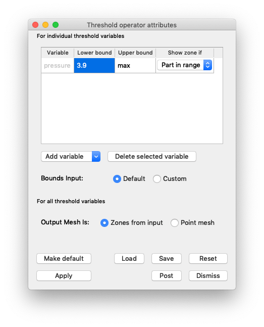
Fig. 7.16 Setting the Isovolume attributes.
Click Apply and dismiss the Threshold attributes Window.
Optionally, open the Pseudocolor attributes Window and change the color table used. These plots use the
Spectralcolor table.Click Draw. You will now see a visualization of the thresholded mesh.
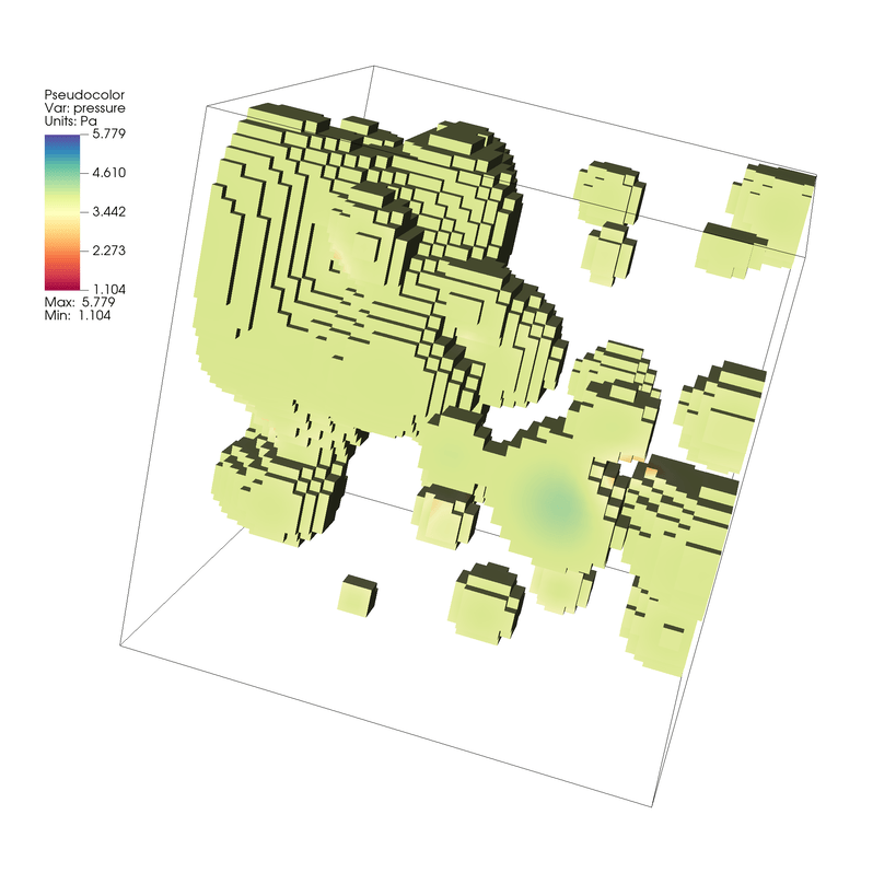
Fig. 7.17 Visualizing our thresholded example of our dataset.
The Threshold operator simply excludes elements from the mesh based on if the threshold criteria is met.
7.2.2. Isovolume
Next, we create a new mesh using the Isovolume operator. We created this in a new viewer window, so we can easily look at both results side-by-side.
Create a new viewer window
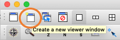
Fig. 7.18 Click to create a new viewer window.
Delete any plots in the new window.
In the plot list, click Add->Pseudocolor->pressure.
In the plot list, click Operators->Selection->Isovolume
Click on the triangle to the left of your Pseudocolor plot and double click Isovolume to open up the Isovolume attributes.
Once you’ve opened the Isovolume attributes, set Variable to pressure and set the Lower bound to 3.9.
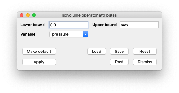
Fig. 7.19 Setting the Isovolume attributes.
Click Apply and dismiss the Threshold attributes Window.
Optionally, open the Pseudocolor attributes Window and change the color table used. These plots use the
Spectralcolor table.Click Draw. You will now see a visualization of the cut mesh.
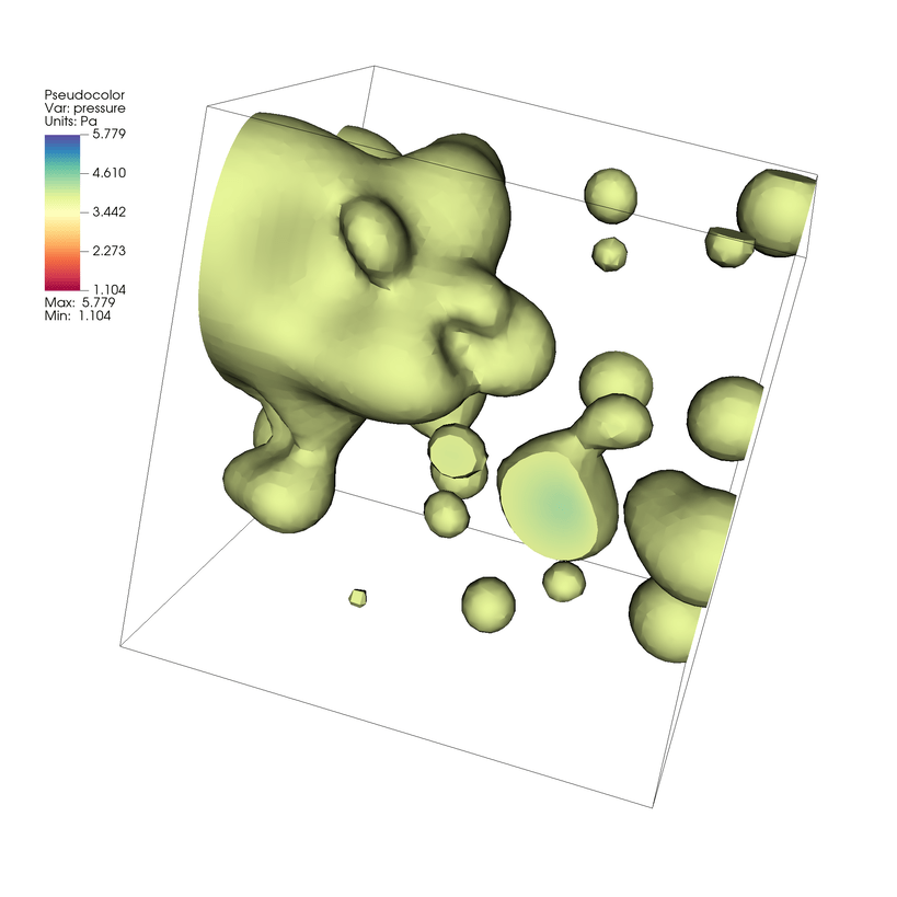
Fig. 7.20 Visualizing an isovolume from our example of our dataset.
The Isovolume cuts the mesh to include volumes between two Isosurfaces.
7.3. Labeling Connected Components with an Expression
The thresholded mesh has a blocky structure and submeshes remain connected at the edges of blocks. The isovolumed mesh has interpolated cuts, which create a smoother result and less connected submeshes. Next, we use the conn_components expression to view and compare connected submeshes for each of these plots.
Open the Expressions Window (Options Menu->Expressions)
Create a new expression named ccl with the definition
conn_components(Mesh).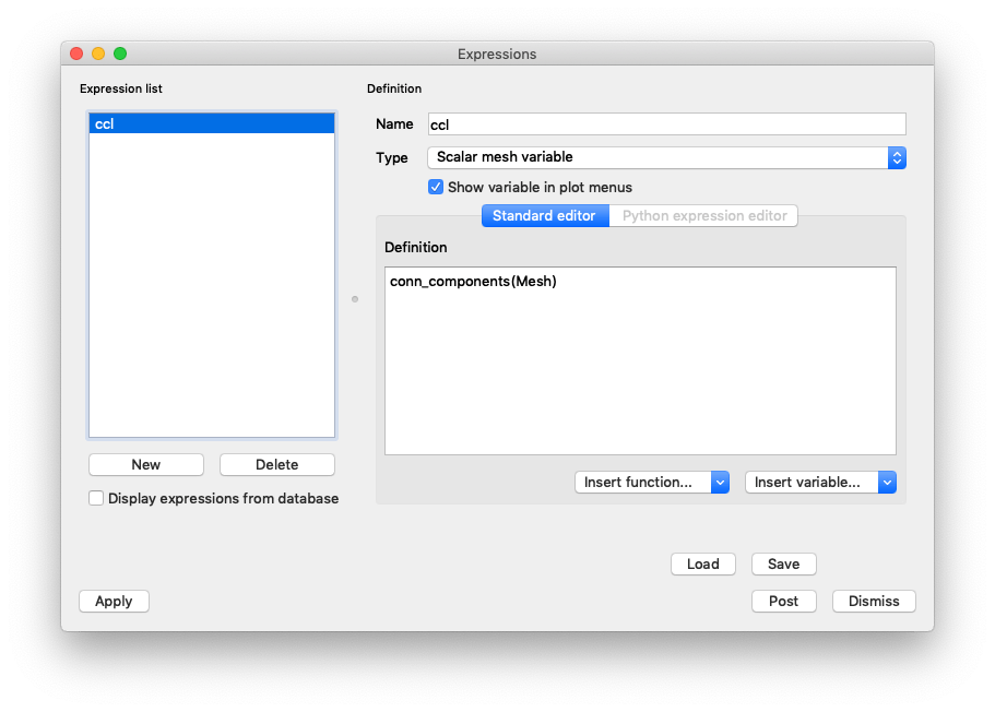
Fig. 7.21 Defining a conn_components expression
Click Apply and dismiss the Expressions Window.
Now we use the ccl expression with our existing pipelines.
7.3.1. Connected Components of Threshold Result
Make Window 1 active (The window with the Threshold operator pipeline)
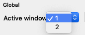
Fig. 7.22 Changing active window to 1
In the plot list, click Operators->Analysis->DeferExpression
Click on the triangle to the left of your Pseudocolor plot, and double click DeferExpression to open up the DeferExpression attributes.
Once you’ve opened the DeferExpression attributes, add ccl to the list of deferred expressions.
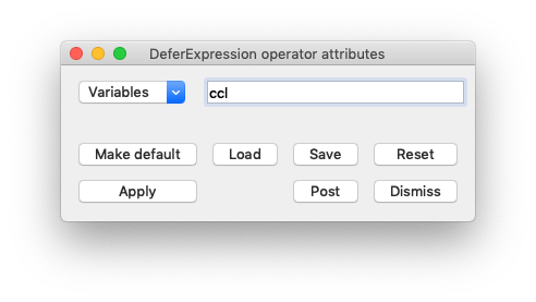
Fig. 7.23 Setting the DeferExpression attributes. This operator instructs VisIt to execute the ccl expression on the Threshold result, instead of the original mesh.
Click Apply and dismiss the DeferExpression attributes Window.
Use the Variables menu to change the active variable to ccl.
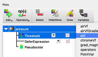
Fig. 7.24 Changing active plot variable to ccl.
Optionally, open the Pseudocolor attributes Window and change the color table used. These plots use the
Spectralcolor table.Click Draw. You will now see the mesh rendered with Connected Component Labels.
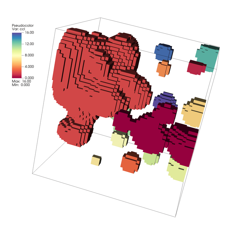
Fig. 7.25 Connected Components of the Threshold Result
We now see a Pseudocolor plot of a new scalar field where each element is associated with its connected component label. In this case we have 17 connected components labeled using ids 0 - 16.
7.3.2. Connected Components of Isovolume Result
Make Window 2 active (The window with the Isovolume operator pipeline )
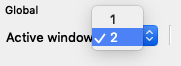
Fig. 7.26 Changing active window to 2
Repeat the steps above to add a DeferExpression operator and set it up to defer the ccl expression.
Use the Variables menu to change the active variable to ccl.
Fig. 7.27 Changing active plot variable to ccl.
Optionally, open the Pseudocolor attributes Window and change the color table used. These plots use the
Spectralcolor table.Click Draw. You will now see the mesh rendered with Connected Component Labels.
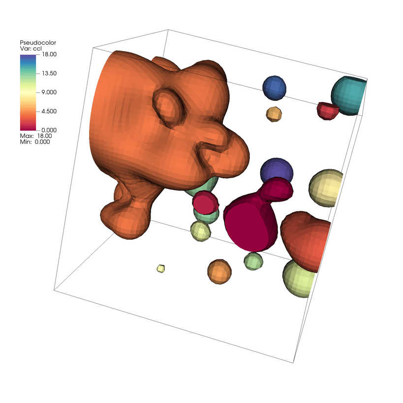
Fig. 7.28 Connected Components of the Isovolume Result
Again, we now have Pseudocolor plot of a new scalar field where each element is associated with its connected component label. In this case we have 19 connected components labeled using ids 0 - 18. You can lock the views between the two windows to compare the differences in the meshes and identify where the connected components differ.
7.4. Using the Connected Component Summary query
The Connected Components Summary query computes and aggregates all component info and optionally writes this data to an okc file (an XMDF File format)
The query returns the following details of each component:
Component Data |
Fields |
|---|---|
Component Id |
comp_label |
Centroid |
comp_x, comp_y, comp_z |
Number of Cells (or Zones) per component |
comp_num_cells |
Area (if the dataset is 2D) |
comp_area |
Volume (if the dataset is 3D or RZ) |
comp_volume |
Variable Sum |
comp_sum |
Weighted Variable Sum |
comp_weighted_sum |
Spatial Bounding Box |
comp_bb_x_min, comp_bb_x_max, comp_bb_y_min, comp_bb_y_max, comp_bb_z_min, comp_bb_z_max |
Number of MPI Tasks spanned by the component |
comp_num_procs |
Next, we use the Connected Components Summary via python on one of our plots to obtain this info.
Launch VisIt’s Command Line Interface (CLI) (Controls Menu->Launch CLI)
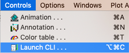
Fig. 7.29 Launch the CLI
Run the following code snippets (Example output below is from the Isovolume case)
Python Snippet
# Execute our connected components query and get the result
Query("Connected Components Summary")
res = GetQueryOutputObject()

# Show names in the results dictionary
print(res.keys())

# Print the array of per component volumes
print(res["comp_volume"])
Output
"Found 19 connected components.\nComponent summary information saved to cc_summary.okc, which can be imported into VisIt"
['comp_bb_x_max', 'comp_bb_z_max', 'comp_sum', 'comp_y', 'comp_num_procs', 'comp_bb_x_min', 'comp_weighted_sum', 'comp_bb_y_min', 'comp_z', 'comp_volume', 'comp_x', 'comp_bb_z_min', 'comp_num_cells', 'connected_component_count', 'comp_bb_y_max']
(37.97730226694259, 3.2019942591930146, 1.610134229606217, 33.371787344299676, 907.2334157190477, 4.499707094552377, 0.9447130410516479, 7.414511301985026, 15.064008190720848, 0.18155970817315392, 3.1918362871108457, 22.247388229041434, 2.625056508686029, 78.24442360391282, 2.4172440068352756, 23.494122927868506, 18.57216353121875, 6.944255799937935, 8.499496779401833)
Python Snippet
# Print all of the results in a ~human friendly way
import json
print(json.dumps(res,indent=2))
Output
Lots of text, so we omit it here!