2. Data Analysis
This section describes two important abstractions in VisIt: Queries and Expressions.
2.1. Queries
2.1.1. What are queries
Queries are a mechanism for performing data analysis. Example use cases include querying for a number or curve that helps to describe the dataset.
2.1.2. Experiment with queries
Go to Controls->Query.
This brings up the Query window.
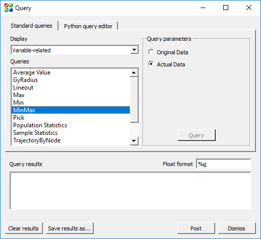
Fig. 2.10 The MinMax query
2.2. Queries over Time
2.2.1. What are queries over time
Queries over time perform analysis through time and generate a time-curve.
2.2.2. Experiment with queries over time
2.2.2.1. Weighted Variable Sum
Go to Controls->Query.
This brings up the Query window.
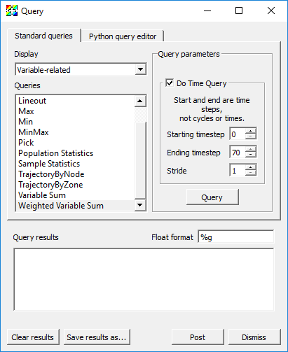
Fig. 2.11 The Weighted Variable Sum query
Go back to the GUI, delete any existing plots, open up “wave.visit”, and make a Pseudocolor plot of pressure.
Find and Highlight Weighted Variable Sum and click Do Time Query.
Options for changing the Starting timestep, Ending timestep and Stride will be available.
Note that these are 0-origin timestate indices and not cycles or times.
Click Query.
The result will be displayed in a new Window. By default the x-axis will be cycle and the y-axis will be the weighted summation of the pressure.
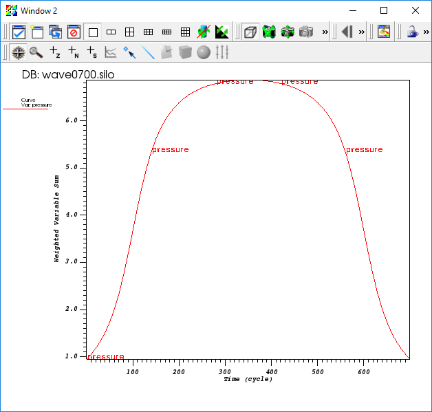
Fig. 2.12 The output of the Weighted Variable Sum query over time
2.2.2.2. Pick
Pick can do multiple-variable time curves.
Make Window 2 active, delete the plot, and make Window 1 active again.
Find and Highlight Pick in the Query window and click Do Time Query to enable time-curve options.
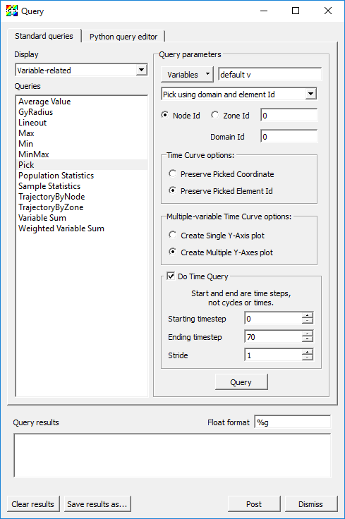
Fig. 2.13 The Pick query
Change the Variables option to add v using the Variables->Scalars dropdown menu.
Select Pick using domain and element Id. Leave the defaults for Node Id and Domain Id as “0”.
Select Preserve Picked Element Id.
Click Query.
The result will be two curves in a single xy plot.
Make Window 2 active, delete the plot, and make Window 1 active again.
Change the Multiple-variable Time Curve options to Create Multiple Y-Axes plot.
Click Query.
The result will be a Multi-curve plot (multiple axes) in Window 2.
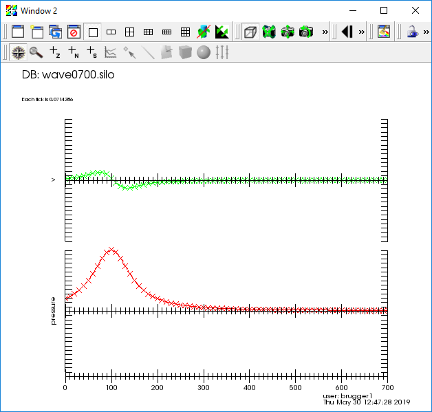
Fig. 2.14 The Pick query output
NOTE: Time Pick can also be performed via the mouse by first setting things up on the Time Pick tab in the Pick window (Controls->Pick).
2.2.3. Changing global options
Go to Controls->Query over time options.
This brings up the QueryOverTime window.
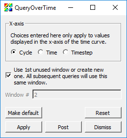
Fig. 2.15 The QueryOverTime window
Here you can change the values displayed in the x-axis for all subsequent queries over time.
You can also change the window used to display time-curves. By default, the first un-used window becomes the time-curve window, and all subsequent time-curves are generated in the same window.
2.3. Built-in queries
VisIt provides a wide variety of built-in queries. See explanations of these here: Built-in queries
2.4. Expressions
Expressions in VisIt create new mesh variables from existing ones. These are also known as derived quantities. VisIt’s expression system supports only derived quantities that create a new mesh variable defined over the entire mesh. Given a mesh on which a variable named pressure is defined, an example of a very simple expression is “2*pressure”. On the other hand, suppose one wanted to sum (or integrate) “pressure” over the entire mesh (maybe the mesh represents some surface area over which a force calculation is desired). Such an operation is not an expression in VisIt because it does not result in a new variable defined over the entire mesh. In this example, summing pressure over the entire mesh results in a single, scalar, number, like “25.6”. Such an operation is supported instead by VisIt’s Variable Sum Query. This tends to be true in general; Expressions define whole mesh variables while Queries define single numerical values (there are, however, some Queries for which this is not strictly true).
2.4.1. A simple algebraic expression, “2*radial”
Open up “noise2d.silo”.
Create a Pseudocolor plot of the variable radial.
Take note of the legend range, “0…28.28”
Go to Controls->Expressions.
Click on New in the bottom left.
This will create an expression and give it a default name, “unnamed1”.
Rename this expression by typing “radial2” into the Name field
Take note of the Type of the variable. By default, VisIt assumes the type of the new variable you are creating is a s scalar mesh variable (e.g. a single numerical value for each node or zone/cell in the mesh). Here, we are indeed creating a scalar variable and so there is no need to adjust the Type. However, in some of the examples that follow, we’ll be creating vector mesh variables and if we don’t specify the correct type, we’ll get an error message.
Place the cursor in the Definition pane of the Expressions dialog.
Type the number “2” followed by the C/C++ language symbol for multiplication, “*”.
Now, you can either type the name “radial” or you can go to the Insert Variable… pulldown menu and find and select the radial variable there (see picture at right).
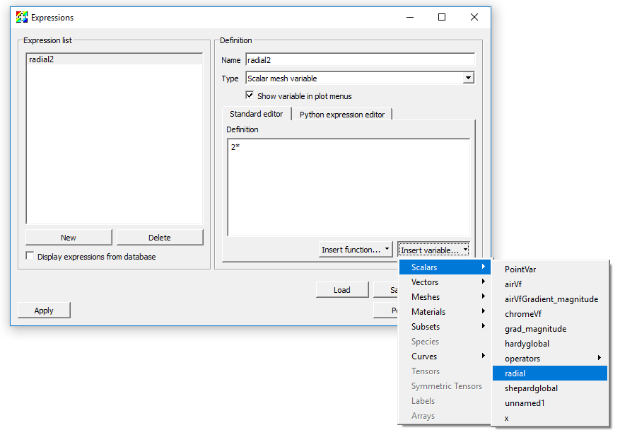
Fig. 2.16 Using the Expressions window Insert variable
Click Apply.
Now, go to the main VisIt GUI Panel to the Variables pulldown.
Note that radial2 now appears in the list of variables there.
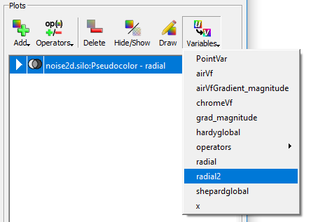
Fig. 2.17 Expression variable appears in the plot menus
Select radial2 from the pull down and click Draw.
Visually, the image will not look any different. But, if you take a close look at the legend you will see it is now showing “0…56.57”.
Visit supports several unary and binary algebraic expressions including
+, -, /, \*, bitwise-^, bitwise-&, sqrt(), abs(), ciel(), floor(), ln(), log10(), exp()
and more.
2.4.2. Accessing coordinates (of a mesh) in expressions
Here, we’ll use the category of Mesh expressions to access the coordinates of a mesh, again, working with “noise2d.silo”.
Go to Controls->Expressions.
Click the New button and name this expression “Coords”.
Set the Type to Vector mesh variable (because coordinates, at least in this 2D example, are a vector quantity).
Put the cursor in the Definition pane.
Go to Insert Function… and find the Mesh category of expressions and then, within it, find the coord function expression.
This should result in the insertion of “coord()” in the Definition pane and place the cursor between the two parenthesis characters.
Note that in almost all cases, the category of Mesh expressions expect one or more mesh variables as operands.
Now, go to Insert Variable… pull down and then to the Meshes submenu and select Mesh.
This should result in Mesh being inserted between the parentheses in the definition.
Click Apply.
Now, we’ll define two scalar expressions for the “X” and “Y” coordinates of the mesh. While still in the Expressions window,
Click New.
Name the new expression “X”.
Note that VisIt’s expression system is case sensitive so “x” and “X” can be different variable names.
Leave the type as Scalar mesh variable
Type into the definition pane, “Coords[0]”
This expression uses the array bracket dereference operator “[]” to specify a particular component of an array. In this case, the array being derefrenced is the vector variable defined by “Coords”.
Note that VisIt’s expression system always numbers its array indices starting from zero.
Click Apply.
Now, repeat these steps to define a “Y” expression for the “Y” coordinates as “Coords[1]”.
Finally, we’ll define the “distance” expression
Click the New button.
Give the new variable the name “Dist” (Type should be Scalar mesh variable).
Type in the definition “sqrt(X*X+Y*Y)”.
Click Apply.
Now, we’ll use the new “Dist” variable we’ve just defined to display some data.
Delete any existing plots from the plot list.
Add a Pseudocolor plot of shepardglobal.
Add an Isovolume operator.
Although this example is a 2D example and so volume doesn’t seem to apply, VisIt’s Isovolume operator performs the equivalent operation for 2D data.
Bring up the Isovolume operator attributes (either expand the plot by clicking on the triangle to the left of its name in the plot list and double clicking on the Isovolume operator there or go to the OpAtts menu and bring up Isovolume operator attributes that way).
Set the variable to Dist.
Set the Lower bound to “5” and the Upper bound to “7”.
Click Apply.
Click Draw.
You should get the picture below. In this picture, we are displaying a Pseudocolor plot of shepardglobal, but Isovolumed by our Dist expression in the range “[5…7]”.
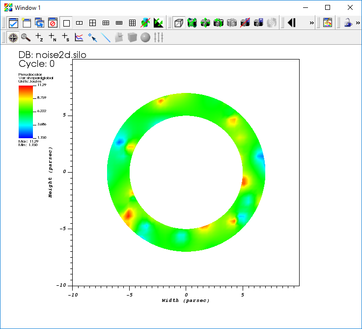
Fig. 2.18 Example of using the radial expression
This example also demonstrates the use of an expression function, coord() to operate on a mesh and return its coordinates as a vector variable on the mesh.
VisIt has a variety of expression functions that operate on a Mesh including area (for 2D meshes), volume (for 3D meshes, revolved_volume (for 2D cylindrically symmetric meshes), zonetype, and more. In addition, VisIt includes the entire suite of Mesh quality expressions from the Verdict Library.
2.4.3. Creating vector and tensor valued variables from scalars
If the database contains scalar variables representing the individual components of a vector or tensor, VisIt’s Expression system allows you to construct the associated vector (or tensor). You create vectors in VisIt’s Expression system using the curly bracket vector compose “{}” operator. For example, using “noise2d.silo” again as an example, suppose we want to compose a Vector valued expression that has “shepardglobal” and “hardyglobal” as components. Here are the steps.
Go to Controls->Expressions.
Click the New button and set Name to “randvec”.
Be sure to also set the Type to Vector mesh variable.
Place the cursor in Definition pane and type “{shepardglobal, hardyglobal}”.
Click Apply.
Go to Plots->Vector.
You should now see randvec appear there as a variable name to plot.
Add the Vector plot of randvec.
In the example above, we used the vector compose operator, “{}” to create a vector variable from multiple scalar variables. We can do the same to create a tensor variable. Recall from calculus that a rank 0 tensor is a scalar, a rank 1 tensor is a vector and a rank 2 tensor is a matrix. So, to create a tensor variable, we use multiple vector compose operators nesting within another vector compose operator. Here, solely for the purposes of illustration (e.g. this isn’t a physically meaningful tensor) we’ll use the “X” and “Y” coordinate component scalars we defined earlier together with the shepardglobal and hardyglobal.
Go to Controls->Expressions.
Click New and set the Name to “tensor”.
Be sure to also set the Type to Tensor mesh variable.
Place the cursor in Definition pane and type “{ {shepardglobal, hardyglobal}, {X,Y} }”.
Note the two levels of curly braces. The outer level is the whole rank 2 tensor matrix and the inner curly braces are each row of the matrix.
Note that you could also have defined the same tensor expression using two vector expressions like so, “{randvec, Coords}”.
Click Apply.
Add a Tensor plot of tensor variable.
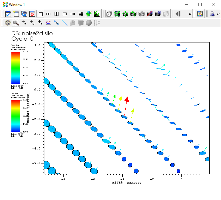
Fig. 2.19 Example of using vector and tensor expressions
2.4.4. Variable compatibility gotchas (tensor rank, centering, mesh)
VisIt will allow you to define expressions that it winds up determining to be invalid later when it attempts to execute those expressions. Some common issues are the mixing of incompatible mesh variables in the same expression without the necessary additional functions to make them compatible.
2.4.4.1. Tensor rank compatibility
For example, what happens if you mix scalar and vector mesh variables (e.g. variables of different Tensor rank) in the same expression? Again, using “noise2d.silo”.
Define the expression, “foo” as “grad+shepardglobal” with the Type Vector mesh variable.
Note that grad is a Vector mesh variable and shepardglobal is a Scalar mesh variable.
Now, attempt to do a Vector plot of foo. This works because VisIt will add the scalar to each component of the vector resulting a new vector mesh variable
But, suppose you instead defined foo to be of Type Scalar mesh variable.
VisIt will allow you to define this expression. But, when you go to plot it, the plot will fail.
As an aside, as you go back and forth between the Expressions window creating and/or adjusting expression definitions, VisIt makes no attempt to keep track of all the changes you’ve made in expressions and automatically update plots as expressions change. You will have to manually clear or delete plots to force VisIt to re-draw plots in which you’ve changed expressions.
In the above example, if on the other hand, you had set type of “foo” to Scalar Mesh Variable, then VisIt would have failed to plot it because it is adding a scalar and a vector variable and the result of such an operation is always a Vector mesh variable. If what you really intended was a scalar mesh variable, then use one of the expression functions that converts a vector to a scalar (e.g. magnitude() function or array dereference operator []) to convert the Vector mesh variable in your expression to a scalar mesh variable. So, “grad[i]+shephardglobal” where “i” is “0” or “1” would work to define a scalar mesh variable. Or, “magnitude(grad)+shepardglobal” would also have worked.
2.4.4.2. Centering compatibility
In “noise2d.silo”, some variables are zone-centered and some are node centered. What happens if you combine these in an expression? VisIt will default to zone centering for the result. If this is not the desired result, use the “recenter()” expression function, where appropriate, to adjust centering of some of the terms in your expression. For example, again using “noise2d.silo”.
Define the Scalar mesh variable expression “bar” as “shepardglobal+airVf”.
For reference, in “noise2d.silo”, “shepardglobal” is node-centered while “airVf” is zone-centered.
Do a Pseudocolor plot of “bar”.
Note that “bar” displays as a zone-centered quantity.
Now, go back to the expression and recenter “airVf” by adjusting the definition to “shepardglobal+recenter(airVf)”.
The recenter() expression function is a toggle in that it will take whatever the variable’s centering is and swap it (node->zone and zone->node).
The recenter() expression function also takes a second argument, a string of one of the values toggle, zonal, nodal to force a particular behavior.
Note that when you click Apply, the current plot of “bar” does not change. You need to manually delete and re-create the plot (or clear and re-draw the plots).
Finally, note that these two expressions…
“shepardglobal+recenter(airVf)”
“recenter(shepardglobal+airVf)”
both achieve a node-centered result. But, each expression is subtly (and numerically) different. The first recenter’s “airVf” to the nodes and then performs the summation operator at each node. In the second, there is an implied recentering of “shepardglobal” to the zones first. Then, the summation operator is applied at each zone center and finally the results are recentered back to the nodes. In all likelihood this results in a numerically lower quality result. The moral is that in a complex series of expressions be sure to take care where you want recentering to occur.
2.4.4.3. Mesh compatibility
In many cases, especially in Silo databases, all the available variables in a database are not always defined on the same mesh. This can complicate matters involving expressions in variables from different meshes.
Just as in the previous two examples of incompatible variables where the solution was to apply some functions to make the variables compatible, we have to do the same thing when variables from different meshes are combined in an expression. The key expression functions which enable this are called Cross Mesh Field Evaluation or CMFE functions. We will only briefly touch on these here. CMFEs will be discussed in much greater detail in a tutorial devoted to that topic.
Again, using “noise2d.silo”
Define the expression “gorf” with definition “PointVar + shepardglobal”.
Note that PointVar is defined on a mesh named PointMesh while shepardglobal is defined on a mesh named Mesh.
Try to do a Pseudocolor plot of “gorfo”. You will get a plot of points and a warning message like this one…
The compute engine running on host somehost.com issued the following warning: In domain 0, your nodal variable “shepardglobal” has 2500 values, but it should have 100. Some values were removed to ensure VisIt runs smoothly.
So, whats happening here? VisIt is deciding to perform the summation operation on the PointVar’s mesh. That mesh consists of 100 points. So, when it encounters the shepardglobal variable (defined on Mesh with 50x50 nodes), it simply ignores any values in “shepardgloabl” after the first 100. Most likely, this is not the desired outcome.
We have two options each of which involves mapping one of the variables onto the other variable’s mesh using one of the CMFE expression functions. We can map shepardglobal onto PointMesh or we can map PointVar onto Mesh. We’ll do both here
2.4.4.4. Mapping shepardglobal onto PointMesh
Define a new expression named “shepardglobal_mapped”.
Go to Insert Function…, then to the Comparisons submenu and select pos_cmfe.
This defines a position based cross-mesh field evaluation function. The other option is a conn_cmfe or connectivity-based which is faster but requires both meshes to be topologically congruent and is not appropriate here.
A template for the arguments to the pos_cmfe will appear in the Definition pane.
Replace “<filename:var>” with “<./noise2d.silo:shepardglobal>”.
This assumes the “noise2d.silo” file is in the same directory from which VisIt was started.
This defines the source or donor variable to be mapped onto a new mesh.
Replace “<meshname>” with “PointMesh”.
This defines the destination or target mesh the variable is to be mapped onto.
Replace “<fill-var-for-uncovered-regions>” with “-1”.
This is needed for position-based CMFE’s because the donor variable’s mesh and target mesh may not always volumetrically overlap 100%. In places where this winds up being the case, VisIt will use this value to fill in.
Now with “shepardglobal_mapped” defined, you can define the desired expression, “PointVar + shepardglobal_mapped” and this will achieve the desired result and is shown below.
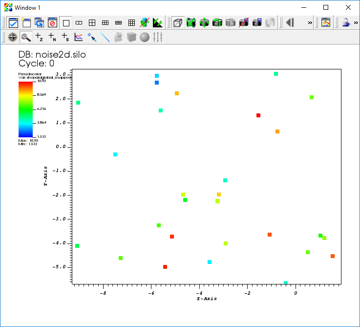
Fig. 2.20 The variable Shepardglobal mapped onto a point mesh
2.4.4.5. Mapping PointVar onto Mesh
To be completed. But, cannot map point mesh onto a volumetric mesh. VisIt always returns zero overlap.
2.4.5. Combining expressions and queries is powerful
Suppose you have a database generated by some application code simulating some object being blown apart. Maybe its a 2D, cylindrically symmetric calculation. Next, suppose the code produced a “density” and “velocity” variable. However, what you want to compute is the total mass of some (portion of) of the object that has velocity (magnitude) greater than some threshold, say 5 meters/second. You can use a combination of Expressions, Queries and the Threshold operator to achieve this.
Mass is “density * volume”. You have a 2D mesh, so how do you get volume from something that has only 2 dimensions? You know the mesh represents a calculation that is cylindrically symmetric (revolved around the y-axis). You can use the revolved_volume() Expression function to obtain the volume of each zone in the mesh. Then, you can multiply the result of revolved_volume() by density to get mass of each zone in the mesh. Once you have that, you can use threshold operator to display only those zones with velocity (magnitude) greater than 5 and then a variable sum query to add up all the mass moving at that velocity.
Here, we demonstrate the steps involved using the “noise2d.silo” database. Because that database does not quite match the problem assumption described in the preceding paragraphs, we simply re-purpose a few of the variables in the database to serve as our density and velocity variables in this example. Namely, we define the expression density as an alias for shephardglobal and velocity as an alias for grad.
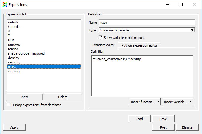
Fig. 2.21 Mass Expression Definition
Here are the steps involved…
Go to Controls->Expressions.
Click New.
Set the Name to “density”.
Make sure the Type is set to Scalar mesh variable.
Set the Definition to “shepardglobal”.
Click Apply.
Click New.
Set the Name to “velocity”.
Make sure the Type is set to Vector mesh variable.
Set the Definition to “grad”.
Click Apply.
Click New.
Set the Name to “mass”.
Make sure the Type is set to Scalar mesh variable.
Set the Definition to “revolved_volume(Mesh) * density”.
Click Apply.
Click the New button again (for a new expression).
Set the Name to “velmag” (for velocity magnitude).
Set the Definition to “magnitude(velocity)”.
Go to Plot->Pseudocolor->mass.
Click Draw.
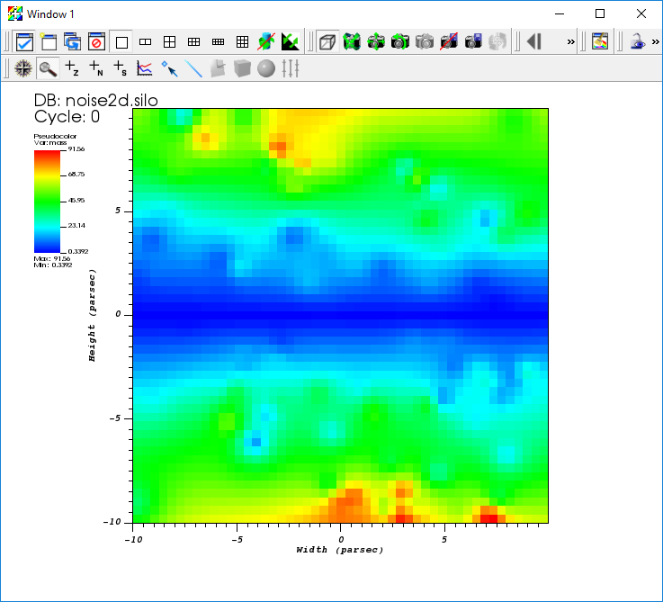
Fig. 2.22 Mass plot
Add Operator->Threshold.
Open the Threshold operator attributes window.
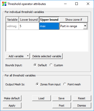
Fig. 2.23 Threshold attributes
Select the default variable and then click Delete selected variable.
Go to Add Variable and select velmag from the list of Scalars.
Set Lower Bound to “5”.
Click Apply.
Now the displayed plot changes to show only those parts of the mesh that are moving with velocity greater than 5.
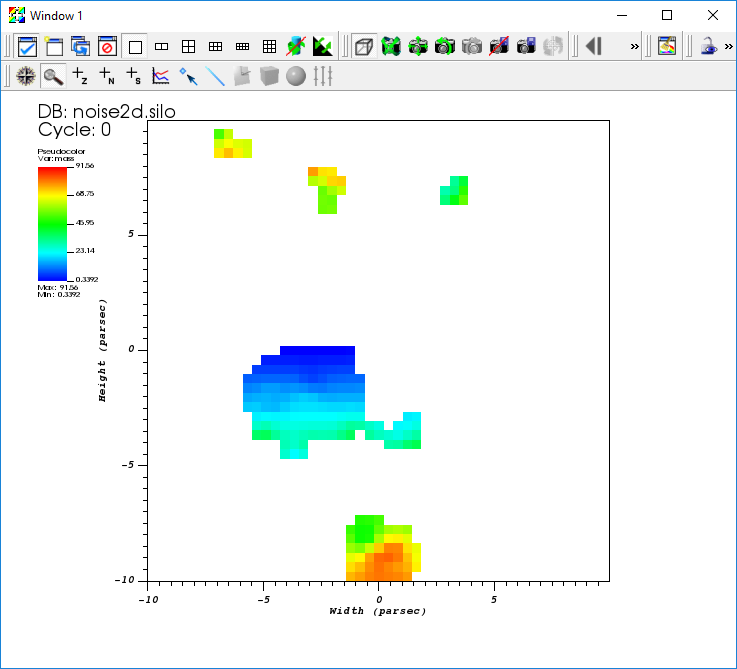
Fig. 2.24 Mass plot after threshold
Go to Controls->Query.
Find the Variable sum query from the list of queries.
Click the Query button. The computed result will be a sum of all the individual zones’ masses in the mesh for those zones that are moving with velocity greater than 5.
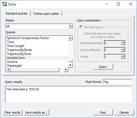
Fig. 2.25 The variable sum query result
2.4.6. Automatic, saved and database expressions
VisIt defines several types of expressions automatically. For all vector variables from a database, VisIt will automatically define the associated magnitude expressions. For unstructured meshes, VisIt will automatically define mesh quality expressions. For any databases consisting of multiple timestates, VisIt will define time derivative expressions. This behavior can be controlled by going to VisIt’s Preferences dialog and enabling or disabling various kinds of automatic expressions.
If you save settings, any expressions you have defined are also saved with the settings. And, they will appear (and sometimes pollute) your menus whether or not they are valid expressions for the currently active database.
Finally, databases are also free to define expressions. In fact, many databases define a large number of expressions for the convenience of their users who often use the expressions in their post-processing workflows. Ordinarily, you never see VisIt’s automatic expressions or a database’s expressions in the Expression window because they are not editable. However, you can check the display expressions from database check box in the Expressions window and VisIt will also show these expressions.