3. Scripting¶

This section describes the VisIt Command Line Interface (CLI).

3.1. Command line interface overview¶

VisIt includes a rich a command line interface that is based on Python 2.7.

There are several ways to use the CLI:

Launch VisIt in a batch mode and run scripts.

Linux: /path/to/visit/bin/visit -nowin -cli -s <script.py>

macOS: /path/to/VisIt.app/Contents/Resources/bin/visit -nowin -cli -s <script.py>

Launch VisIt so that a visualization window is visible and interactively issue CLI commands.
Use both the standard GUI and CLI simultaneously.

3.2. Launching the CLI¶

We will focus on the use case where we have the graphical user interface and CLI running simultaneously.

To launch the CLI from the graphical user interface:

Go to Controls->Command.

This will bring up the Commands window. The Command window provides a text editor with Python syntax highlighting and an Execute button that tells VisIt to execute the script. Finally, the Command window lets you record your GUI actions into Python code that you can use in your scripts.

3.3. A first action in the CLI¶

Open “example.silo” in the GUI if it not already open.

Cut-and-paste the following Python commands into the first tab of the Commands window.

AddPlot("Pseudocolor", "temp")
# You will see the active plots list in the GUI update, since the CLI and GUI communicate.
DrawPlots()
# You will see your plot.

Click Execute.

3.4. Tips about Python¶

Python is whitespace sensitive! This is a pain, especially when you are cut-n-pasting things.

Python has great constructs for control and iteration, here are some examples:

for i in range(100):
   # use i

# strided range
for i in range(0,100,10):
   # use i

if (cond):
 # stmt

import sys
...
sys.exit()

3.5. Example scripts¶

We will be using Python scripts in each of the following sections: You can get execute them by:

Cut-n-paste-ing them into a tab in the Commands window and executing it.

For all of these scripts, make sure “example.silo” is currently open unless otherwise noted.

3.5.1. Setting attributes¶

Each of VisIt’s Plots and Operators expose a set of attributes that control their behavior. In VisIt’s GUI, these attributes are modified via options windows. VisIt’s CLI provides a set of simple Python objects that control these attributes. Here is an example setting the minimum and maximum for the Pseudocolor plot

DeleteAllPlots()
AddPlot("Pseudocolor", "temp")
DrawPlots()
p = PseudocolorAttributes()
p.minFlag = 1
p.maxFlag = 1
p.min = 3.5
p.max = 7.5
SetPlotOptions(p)

3.5.2. Animating an isosurface¶

This example demonstrates sweeping an isosurface operator to animate the display of a range of isovalues from “example.silo”.

DeleteAllPlots()
AddPlot("Pseudocolor", "temp")
iso_atts = IsosurfaceAttributes()
iso_atts.contourMethod = iso_atts.Value
iso_atts.variable = "temp"
AddOperator("Isosurface")
DrawPlots()
for i in range(30):
   iso_atts.contourValue = (2 + 0.1*i)
   SetOperatorOptions(iso_atts)
   # For moviemaking, you'll need to save off the image
   # SaveWindow()

3.5.3. Using all of VisIt’s building blocks¶

This example uses a Pseudocolor plot with a ThreeSlice operator applied to display temp on the exterior of the grid along with streamlines of the gradient of temp.

Note that the script below may not work the first time you execute it. In that case delete all the plots and execute the script again.

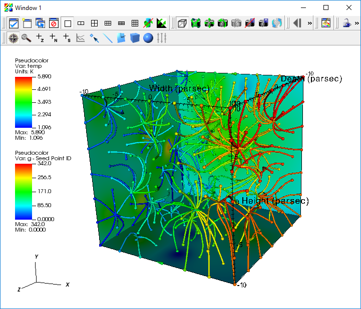
../_images/Scripting-StreamlineOutput.png

Fig. 3.74 Streamlines¶

# Clear any previous plots
DeleteAllPlots()
# Create a plot of the scalar field 'temp'
AddPlot("Pseudocolor","temp")
# Slice the volume to show only three
# external faces.
AddOperator("ThreeSlice")
tatts = ThreeSliceAttributes()
tatts.x = -10
tatts.y = -10
tatts.z = -10
SetOperatorOptions(tatts)
DrawPlots()
# Find the maximum value of the field 'temp'
Query("Max")
val = GetQueryOutputValue()
print("Max value of 'temp' = ", val)

# Create a streamline plot that follows
# the gradient of 'temp'
DefineVectorExpression("g","gradient(temp)")
AddPlot("Pseudocolor", "operators/IntegralCurve/g")
iatts = IntegralCurveAttributes()
iatts.sourceType = iatts.SpecifiedBox
iatts.sampleDensity0 = 7
iatts.sampleDensity1 = 7
iatts.sampleDensity2 = 7
iatts.dataValue = iatts.SeedPointID
iatts.integrationType = iatts.DormandPrince
iatts.issueStiffnessWarnings = 0
iatts.issueCriticalPointsWarnings = 0
SetOperatorOptions(iatts)

# set style of streamlines
patts = PseudocolorAttributes()
patts.lineType = patts.Tube 
patts.tailStyle = patts.Spheres
patts.headStyle = patts.Cones
patts.endPointRadiusBBox = 0.01
SetPlotOptions(patts)

DrawPlots()

3.5.4. Creating a movie of animated streamline paths¶

This example extends the “Using all of VisIt’s Building Blocks” example by

animating the paths of the streamlines
saving images of the animation
finally, encoding those images into a movie

(Note: Encoding requires ffmpeg is installed and available in your PATH)

# import visit_utils, we will use it to help encode our movie
from visit_utils import *
 
# Set a better view
ResetView()
v = GetView3D()
v.RotateAxis(0,44)
v.RotateAxis(1,-23)
SetView3D(v)
 
# Disable annotations
aatts = AnnotationAttributes()
aatts.axes3D.visible = 0
aatts.axes3D.triadFlag = 0
aatts.axes3D.bboxFlag = 0
aatts.userInfoFlag = 0
aatts.databaseInfoFlag = 0
aatts.legendInfoFlag = 0
SetAnnotationAttributes(aatts)
 
# Set basic save options
swatts = SaveWindowAttributes()
#
# The 'family' option controls if visit automatically adds a frame number to 
# the rendered files. For this example we will explicitly manage the output name.
#
swatts.family = 0
#
# select PNG as the output file format
#
swatts.format = swatts.PNG 
#
# set the width of the output image
#
swatts.width = 1024 
#
# set the height of the output image
#
swatts.height = 1024
 

 
####
# Crop streamlines to render them at increasing time values over 50 steps
####
iatts.cropValue = iatts.Time 
iatts.cropEndFlag = 1
iatts.cropBeginFlag = 1
iatts.cropBegin = 0
for ts in range(0,50):
    # set the integral curve attributes to change the where we crop the streamlines
    iatts.cropEnd = (ts + 1) * .5
    
    # update streamline attributes and draw the plot
    SetOperatorOptions(iatts)
    DrawPlots()
    #before we render the result, explicitly set the filename for this render
    swatts.fileName = "streamline_crop_example_%04d.png" % ts
    SetSaveWindowAttributes(swatts)
    # render the image to a PNG file
    SaveWindow()
 
################
# use visit_utils.encoding to encode these images into a "mp4" movie
#
# The encoder looks for a printf style pattern in the input path to identify the frames of the movie.
# The frame numbers need to start at 0. 
# 
# The encoder selects a set of decent encoding settings based on the extension of the
# the output movie file (second argument). In this case we will create a "mp4" file. 
# 
# Other supported options include ".mpg", ".mov". 
#   "mp4" is usually the best choice and plays on all most all platforms (Linux ,OSX, Windows).
#   "mpg" is lower quality, but should play on any platform.
#
# 'fdup' controls the number of times each frame is duplicated. 
#  Duplicating the frames allows you to slow the pace of the movie to something reasonable. 
#
################
 
input_pattern = "streamline_crop_example_%04d.png"
output_movie = "streamline_crop_example.mp4"
encoding.encode(input_pattern,output_movie,fdup=4)

3.5.5. Rendering each time step of a dataset to a movie¶

This example assumes the “aneurysm.visit” is already opened.

Create a plot, render all timesteps and encode a movie.

(Note: Encoding requires that ffmpeg is installed and available in your PATH)

# import visit_utils, we will use it to help encode our movie
from visit_utils import *
DeleteAllPlots()

AddPlot("Pseudocolor","pressure")
DrawPlots()
 
# Set a better view
ResetView()
v = GetView3D()
v.RotateAxis(1,90)
SetView3D(v)
 
# get the number of timesteps
nts = TimeSliderGetNStates()
 
# set basic save options
swatts = SaveWindowAttributes()
#
# The 'family' option controls if visit automatically adds a frame number to 
# the rendered files. For this example we will explicitly manage the output name.
#
swatts.family = 0
#
# select PNG as the output file format
#
swatts.format = swatts.PNG 
#
# set the width of the output image
#
swatts.width = 1024 
#
# set the height of the output image
#
swatts.height = 1024

#the encoder expects file names with an integer sequence
# 0,1,2,3 .... N-1

file_idx = 0

for ts in range(0,nts,10): # look at every 10th frame
    # Change to the next timestep
    TimeSliderSetState(ts)
    #before we render the result, explicitly set the filename for this render
    swatts.fileName = "blood_flow_example_%04d.png" % file_idx
    SetSaveWindowAttributes(swatts)
    # render the image to a PNG file
    SaveWindow()
    file_idx +=1

################
# use visit_utils.encoding to encode these images into a "mp4" movie
#
# The encoder looks for a printf style pattern in the input path to identify the frames of the movie.
# The frame numbers need to start at 0. 
# 
# The encoder selects a set of decent encoding settings based on the extension of the
# the output movie file (second argument). In this case we will create a "mp4" file. 
# 
# Other supported options include ".mpg", ".mov". 
#   "mp4" is usually the best choice and plays on all most all platforms (Linux ,OSX, Windows).
#   "mpg" is lower quality, but should play on any platform.
#
# 'fdup' controls the number of times each frame is duplicated. 
#  Duplicating the frames allows you to slow the pace of the movie to something reasonable.
#
################
 
input_pattern = "blood_flow_example_%04d.png"
output_movie = "blood_flow_example.mp4"
encoding.encode(input_pattern,output_movie,fdup=4)

3.5.6. Animating the camera¶

def fly():
    # Do a pseudocolor plot of u.
    DeleteAllPlots()
    AddPlot('Pseudocolor', 'temp')
    AddOperator("Clip")
    c = ClipAttributes()
    c.funcType = c.Sphere  # Plane, Sphere
    c.center = (0, 0, 0)
    c.radius = 10
    c.sphereInverse = 1
    SetOperatorOptions(c)
    DrawPlots()
 
    # Create the control points for the views.
    c0 = View3DAttributes()
    c0.viewNormal = (0, 0, 1)
    c0.focus = (0, 0, 0)
    c0.viewUp = (0, 1, 0)
    c0.viewAngle = 30
    c0.parallelScale = 17.3205
    c0.nearPlane = 17.3205
    c0.farPlane = 81.9615
    c0.perspective = 1
 
    c1 = View3DAttributes()
    c1.viewNormal = (-0.499159, 0.475135, 0.724629)
    c1.focus = (0, 0, 0)
    c1.viewUp = (0.196284, 0.876524, -0.439521)
    c1.viewAngle = 30
    c1.parallelScale = 14.0932
    c1.nearPlane = 15.276
    c1.farPlane = 69.917
    c1.perspective = 1
 
    c2 = View3DAttributes()
    c2.viewNormal = (-0.522881, 0.831168, -0.189092)
    c2.focus = (0, 0, 0)
    c2.viewUp = (0.783763, 0.556011, 0.27671)
    c2.viewAngle = 30
    c2.parallelScale = 11.3107
    c2.nearPlane = 14.8914
    c2.farPlane = 59.5324
    c2.perspective = 1
 
    c3 = View3DAttributes()
    c3.viewNormal = (-0.438771, 0.523661, -0.730246)
    c3.focus = (0, 0, 0)
    c3.viewUp = (-0.0199911, 0.80676, 0.590541)
    c3.viewAngle = 30
    c3.parallelScale = 8.28257
    c3.nearPlane = 3.5905
    c3.farPlane = 48.2315
    c3.perspective = 1
 
    c4 = View3DAttributes()
    c4.viewNormal = (0.286142, -0.342802, -0.894768)
    c4.focus = (0, 0, 0)
    c4.viewUp = (-0.0382056, 0.928989, -0.36813)
    c4.viewAngle = 30
    c4.parallelScale = 10.4152
    c4.nearPlane = 1.5495
    c4.farPlane = 56.1905
    c4.perspective = 1
 
    c5 = View3DAttributes()
    c5.viewNormal = (0.974296, -0.223599, -0.0274086)
    c5.focus = (0, 0, 0)
    c5.viewUp = (0.222245, 0.97394, -0.0452541)
    c5.viewAngle = 30
    c5.parallelScale = 1.1052
    c5.nearPlane = 24.1248
    c5.farPlane = 58.7658
    c5.perspective = 1
 
    c6 = c0
 
    # Create a tuple of camera values and x values. The x values are weights
    # that help to determine where in [0,1] the control points occur.
    cpts = (c0, c1, c2, c3, c4, c5, c6)
    x=[]
    for i in range(7):
        x = x + [float(i) / float(6.)]
 
    # Animate the camera. Note that we use the new built-in EvalCubicSpline
    # function which takes a t value from [0,1] a tuple of t values and a tuple
    # of control points. In this case, the control points are View3DAttributes
    # objects that we are using to animate the camera but they can be any object
    # that supports +, * operators.
    nsteps = 100
    for i in range(nsteps):
        t = float(i) / float(nsteps - 1)
        c = EvalCubicSpline(t, x, cpts)
        c.nearPlane = -34.461
        c.farPlane = 34.461
        SetView3D(c)
        # For moviemaking...
        # SaveWindow()
 
fly()

3.5.7. Automating data analysis¶

def TakeMassPerSlice():
   DeleteAllPlots()
   AddPlot("Pseudocolor", "chromeVf")
   AddOperator("Slice")
   DrawPlots()
   f = open("mass_per_slice.ultra", "w")
   f.write("# mass_per_slice\n")
   for i in range(50):
     intercept = -10 + 20*(i/49.)
     s = SliceAttributes()
     s.axisType = s.XAxis
     s.originType = s.Intercept
     s.originIntercept = intercept
     SetOperatorOptions(s)
     Query("Weighted Variable Sum")
     t2 = GetQueryOutputValue()
     str = "%25.15e %25.15e\n" %(intercept, t2)
     f.write(str)
   f.close()
 
TakeMassPerSlice()
DeleteAllPlots()
OpenDatabase("mass_per_slice.ultra")
AddPlot("Curve", "mass_per_slice")
DrawPlots()

3.5.8. Extracting a per-material aggregate value at each timestep¶

####################
# Example that demonstrates looping over a dataset
# to extract an aggregate value at each timestep.
#
#  visit -nowin -cli -s listing_8_extracting_aggregate_values.py wave.visit pressure wave_pressure_out
####################
 
import sys
from visit_utils import *
 
def setup_plot(dbname,varname, materials = None):
    """
    Create a plot to query.
    """
    OpenDatabase(dbname)
    AddPlot("Pseudocolor",varname)
    if not materials is None:
        TurnMaterialsOff()
        # select the materials (by id )
        # example 
        #  materials = [ "1", "2", "4"]
        for material in materials:
            TurnMaterialsOn(materials)
    DrawPlots()
 
def extract_curve(varname,obase,stride=1):
    """
    Loop over all time steps and extract a value at each one.
    """
    f = open(obase + ".ult","w")
    f.write("# %s vs time\n" % varname)
    nts = TimeSliderGetNStates()
    for ts in range(0,nts,stride):
        print("processing timestate: %d" % ts)
        TimeSliderSetState(ts)
        tval = query("Time")
        # sums plotted variable scaled by 
        #   area (2D mesh), 
        #   revolved_volume (2D RZ mesh, or 
        #   volume (3D mesh)
        rval = query("Weighted Variable Sum")
        # or you can use other queries, such as max:
        # mval = query("Maximum")
        res = "%s %s\n" % (str(tval),str(rval))
        print(res)
        f.write(res)
    f.close()
 
 
def open_engine():
    # to open an parallel engine
    #  inside of an mxterm or batch script use:
    engine.open(method="slurm")
    #  outside of an mxterm or batch script
    # engine.open(nprocs=21)
 
def main():
    nargs = len(sys.argv)
    if nargs < 4:
        usage_msg = "usage: visit -nowin -cli -s visit_extract_curve.py "
        usage_msg += "{databsase_name} {variable_name} {output_file_base}"
        print(usage_msg)
        sys.exit(-1)
    # get our args
    dbname  = sys.argv[1]
    varname = sys.argv[2]
    obase   = sys.argv[3]
    # if you need a parallel engine:
    # open_engine()
    setup_plot(dbname,varname)
    extract_curve(varname,obase)
 
 
if __visit_script_file__ == __visit_source_file__:
    main()
    sys.exit(0)

3.6. Recording GUI actions to Python scripts¶

VisIt’s Commands window provides a mechanism to translate GUI actions into their equivalent Python commands.

Open the Commands Window by selecting ‘’Controls Menu->Command’’

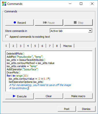
Fig. 3.75 The Commands window¶

Click the Record button.
Perform GUI actions.
Return to the Commands Window.
Select a tab to hold the python script of your recorded actions.
Click the Stop button.
The equivalent Python script will be placed in the tab in the Commands window.

Note that the scripts are very verbose and contain some unnecessary commands, which can be edited out.

3.7. Learning the CLI¶

Here are some tips to help you quickly learn how to use VisIt’s CLI:

From within VisIt’s python CLI, you can type “dir()” to see the list of all commands.

Sometimes, the output from “dir()” within VisIt’s python CLI is a little hard to look through. So, a useful thing on Linux to get a nicer list of methods is the following shell command (typed from outside VisIt’s python CLI)…
echo "dir()" | visit -cli -nowin -forceinteractivecli | tr ',' '\n' | tr -d " '" | sort
Or, if you are looking for CLI functions having to do with a specific thing…
echo "dir()" | visit -cli -nowin -forceinteractivecli | tr ',' '\n' | tr -d " '" | grep -i material

You can learn the syntax of a given method by typing “help(MethodName)”

Type “help(AddPlot)” in the Python interpreter.

Use the GUI to Python recording featured outlined in Recording GUI actions to Python scripts.
Use ‘’WriteScript()’’ function, which will create a python script that describes all of your current plots.

For more details, see WriteScript.

When you have a Python object, you can see all of its attributes by printing it.

s = SliceAttributes()
print s
# Output:
originType = Intercept  # Point, Intercept, Percent, Zone, Node
originPoint = (0, 0, 0)
originIntercept = 0
originPercent = 0
originZone = 0
originNode = 0
normal = (0, -1, 0)
axisType = YAxis  # XAxis, YAxis, ZAxis, Arbitrary, ThetaPhi
upAxis = (0, 0, 1)
project2d = 1
interactive = 1
flip = 0
originZoneDomain = 0
originNodeDomain = 0
meshName = "default"
theta = 0
phi = 0

See the section on apropos, help and lsearch for more information on finding stuff in VisIt’s CLI.

3.8. Advanced features¶

You can set up your own buttons in the VisIt gui using the CLI. See VisIt Run Commands (RC) File.
You can set up callbacks in the CLI that get called whenever events happen in VisIt. See Python callbacks.
You can create your own custom Qt GUI that uses VisIt for plotting. See PySide recipes.